Linear or nonlinear with respect to what?

Overview
I’m teaching a partial differential equations (PDEs) course in the mathematics department at the moment. A typical ‘gimme’ question for assignments and tests is to get the students to classify a given equation as linear or nonlinear (most of the theory we develop in the course is for linear equations so we need to know what this means). Since we aim to introduce the students to a bit of operator theory we often switch back and forward between talking about linear/nonlinear PDEs and linear/nonlinear operators.

One of the students noticed that this introduced some ambiguity into our classification problem and asked a great question. I think it illustrates a useful general point about terminology like linear vs nonlinear and how these terms can be misleading or ambiguous. So here’s the question and my attempt at clarifying the ambiguity.

The question
It’s my understanding that a PDE is linear if we can write it in the form Lu = f(x,t), where L is a linear differential operator.

If we are given a PDE that looks like Au = 0 for some differential operator A and asked to show that the PDE is nonlinear, I can (probably) show that A is not a linear differential operator. However this doesn’t necessarily imply that you cannot rearrange the equation in such a way to make it linear.

For example the operator A defined by

Au = (u^2+1)u_t+(u^2+1)u_{xx}

is not a linear differential operator. However the equation Au = 0 is the same as u_t + u_{xx} = 0, and the differential operator B defined by Bu = u_t + u_{xx} is linear.

So (I believe I’m correct in saying this), the original PDE is linear, because it can be rewritten in this form Lu = f(x,t) for some linear differential operator L and function f(x,t).

My question is what sort of working are we expected to show, if we aim to prove the PDE Au=0 is not linear? For the purposes of the assignment does it suffice to prove that A is not linear?

My response
Here was my response and attempt to clarify (corrections/comments welcome!).

Great question!

As you’ve noticed there is some ambiguity when we move back and forward between talking about equations and operators. This is to be expected since a function (e.g. an operator) is a different type of mathematical object to an equation

For example the function f:x \mapsto x^2 is a different ‘object’ to the equation x^2 = 0.

You’ve correctly noticed that if we can write a differential equation as Lu = f where L is some linear operator then the differential equation is also called linear. Unfortunately, again as you’ve noticed, this definition makes it hard to decide when an equation is nonlinear as you may be able to write a linear equation in terms of a nonlinear operator with the right choice of f. This is because the negation of ‘there exists’ a linear operator is ‘there doesn’t exist a linear operator’.

So proving that an equation is linear is easy using the operator definition – we just find any linear operator that works.

On the other hand, proving that an equation is nonlinear is harder using this definition – it would require showing all operators for which Au = f are nonlinear.

This seems too hard to do directly, so let’s reformulate it in an equivalent but easier-to-use way.

We want to keep our definitions of linear and nonlinear as close as possible for the two cases of operators and equations.

So, how about:

Improved definitions

An operator acting on u is linear iff L(au+bv) = aL(u) + bL(v) for any u and v in the operator’s domain and constants a, b.

and

Given an equation written in the from Au = f for some operator A and forcing function f, the equation is linear iff A(au+bv) = aA(u) + bA(v) for any two solutions u, v to the equation Au = f.

I think this definition should cover your example (try it! Note that it is slightly subtle how this makes a difference! But, basically, we get to use the f = 0 in the equation case now).

Also note that:

The function definition now explicitly talks about linearity with respect to how it operates on objects in its domain while the equation definition talks explicitly about behaviour with respect to solutions to that equation. This seems natural given the different ‘nature’ of ‘functions’ and ‘equations’.

Does that make sense?

Morally speaking
I think the broader lesson is that terms like linear/nonlinear are relative to the specific mathematical representation chosen and how we interact with that representation. A ‘system’ is not really intrinsically linear or nonlinear, rather an ‘action’ (or function or operator or process) is linear or nonlinear with respect to a specific set of ‘objects’ or ‘measurements’ or ‘perturbations’ or whatever. This needs to be made explicit for an unambiguous classification to be carried out.

Generalisation
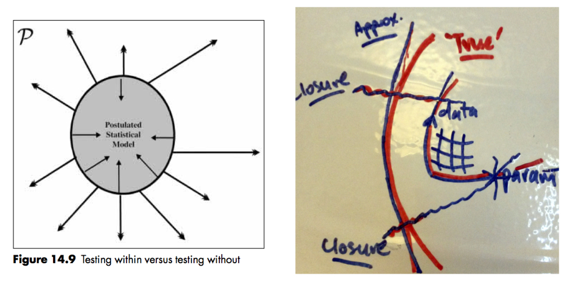
Perhaps generalising too far, something like this came up in some recent ‘philosophical’ discussions I’ve been having over at Mayo’s blog (and was also at the heart of another scientific disagreement I once had with an experimentalist about interpreting aquaporin knockout experiments…).

For example, it has been pointed out that while ‘chaos’ is typically associated with (usually finite-dimensional) nonlinear systems, there are examples of infinite-dimensional linear systems that exhibit all the hallmarks of chaos – see e.g. ‘Linear vs nonlinear and infinite vs finite: An interpretation of chaos‘ by Protopopescu for just one example. So, changing the underlying ‘objects’ used in the representation changes the classification as ‘linear’ or ‘nonlinear’ or, as Protopopescu states

Linear and nonlinear are somewhat interchangeable features, depending on scale and representation…chaotic behavior occurs… when we have to deal with infinite amounts of information at a finite level of operability. In this sense, even the most deterministic system will behave stochastically due to unavoidable and unknown truncations of information.

This theme appears again and again at various levels of abstraction – e.g. we saw it in a high-school math problem where a singularity (a type of ‘lack of regularity’) arose (which we interpreted as) due to an incompatibility between a regular higher-dimensional system and a constraint restricting that system to a lower-dimensional space. (Compare the abstract operator itself with the operator + equating it to zero to get an equation.) We were faced with the choice of a regular but underdetermined system that required additional information for a unique solution or a ‘unique’ but singular (effectively overdetermined) system. Similarly other ‘irregular’ behaviour like ‘irreversibility’ can often be thought of as arising due to a combination of ‘reversible’ (symmetric/regular etc) microscopic laws + asymmetric boundary conditions/incomplete measurement constraints. Similar connections between ‘low/high dimensional’ systems and ‘stable/unstable’ systems are discussed by Kuehn in ‘The curse of instability‘.

To me this presents a helpful heuristic decomposition of models of the world into two-level decompositions like ‘irregular nature’ -> ‘regular, high-dimensional nature’ + ‘limited accessibility to nature’ (h/t Plato) or ‘internal dynamics’ + ‘boundary conditions’, ‘reversible laws’ + ‘irreversible reductions/coarse-graining’ etc. Note also that, on this view, ‘infinite’ and ‘finite’ are effectively ‘relative’, ‘structural’ concepts – if our ‘access’ to the ‘real world’ is always and instrinsically limited it leads us to perceive the world as effectively infinite (in some sense) regardless of whether the world is ‘actually’ infinite. You still can’t really avoid ‘structural infinities’ –  e.g. continuous transformations – though.

It seems clear that this also inevitably introduces ‘measurement problems’ that aren’t that dissimilar to those considered to be intrinsic to quantum mechanics into even ‘classical’ systems, and leads to ideas like conceiving of ‘stochastic’ models as ‘chaotic deterministic’ systems and vice-versa.

Recent reading: a miscellany of slightly obscure things

Sometimes I forget which things I’m currently reading (i.e. dipping in and out of). So, here are a few notes, mainly to myself and mainly about books and more obscure sources than the usual current research papers.

A couple of things on category theory: Category Theory for the Sciences by Spivak and Sets for Mathematics by Lawvere and Rosebrugh. (Also Mathematical Physics by Geroch, but that is more of a broad coverage of essential mathematics using category theory than a book introducing/studying category theory itself.) Really enjoying both. Would like to code up some of the content of Spivak to illustrate the main ideas.

A few things on mathematical biology/physiology etc (mainly for work/background I should know but have either forgotten or not learned). Mathematical Physiology by Keener and Sneyd (the latter being my old PhD supervisor). Free Energy Transduction and Biochemical Cycle Kinetics by Hill (as well as the older, longer version). An underrated book, I need to summarise the best bits at some point. Basic Principles of Membrane Transport by Schultz. Another great classic, helped me a lot during my PhD. Both a bit old but the main thing that seems to have changed is that we have actually identified a lot of the proteins behind the mechanisms originally predicted on based on coarse information and largely theoretical modelling!

Stochastic Modelling for Systems Biology by Wilkinson, Chemical Biophysics by Qian and Beard and Stochastic Process for Physics and Chemistry by van Kampen. Good complements to the above books, generally more focused on stochastic aspects, but still similar concepts. See also the papers Entropy Production in Mesoscopic Stochastic Thermodynamics: Nonequilibrium Kinetic Cycles Driven by Chemical Potentials, Temperatures, and Mechanical Forces by Qian et al. as well as Contact Geometry of Mesoscopic Thermodynamics and Dynamics by Grmela. Also, the book Statistical Thermodynamics of Nonequilibrium processes by Keizer. Should summarise the various key concepts and how to think about ‘mesoscopic’ processes in biology.

A few references on mechanics: some point particle stuff (want to use in some applications), also differential geometry, symmetry etc. Introduction to Physical Modelling by Wellstead (mainly interested in the ‘mobility analogy’). The Variational Principles of Mechanics by Lanczos (a classic!). Analytical Dynamics by Udwadia and Kalaba. Nonholonomic Mechanics and Control by Bloch et al. First Steps in Differential Geometry: Riemannian, Contact, Symplectic by McInerney. Discrete Differential Geometry: An Applied Introduction by Grinspun et al. Foundations of Mechanics by Abraham and Marsden. Introduction to Mechanics and Symmetry by Ratiu and Marsden. Mathematical Foundations of Elasticity by Marsden and Hughes. Also the paper: ‘On the Nature of Constraints for Continua Undergoing Dissipative Processes’ by Rajagopal and Srinivasa.

Dynamical systems (research and teaching – solution and analysis methods): Numerical Continuation Methods for Dynamical Systems by Krauskopf, Osinga and Galan-Vioque. Recipes for Continuation by Dankowicz and Schilder. Stability, Instability and Chaos by Glendinning. Nonlinear Systems by Drazin. Elements of Applied Bifurcation Theory by Kuznetsov. Applications of Lie Groups to Differential Equations by Olver. Scaling by Barenblatt. Renormalization Methods: A Guide For Beginners by McComb. Multiple Time Scale Dynamics by Kuehn.

Measure, Integral and Probability by Capinski and Kopp, Integral, Measure and Derivative by Shilov and Gurevich and Hilbert Space Methods in Probability and Statistical Inference by Small and McLeish (see also Functional Analysis by Muscat). Probability via Expectation By Whittle. Functional Analysis for Probability and Stochastic Processes: An Introduction by Bobrowski. Trying to decide on my preferred abstract framework for thinking about these topics. Each presents a slightly different perspective, each has its strengths and weaknesses. Will have to write a ‘compare and contrast’ to help me decide. I’ve pretty well decided on the functional analysis point of view. Update: see also Differential Geometry and Statistics by Amari and Differential Geometry and Statistics by Murray and Rice. So basically: functional analysis + differential geometry seems to be the way to go. Same as for mechanics.

Related to the above, a few books (and a paper or two) on inverse problems, parameter estimation, Bayesian inference and numerical approximation. Data Assimilation: A Mathematical Introduction by Law, Stuart and Zygalakis. Inverse Problems: A Bayesian Perspective by Stuart. Mapping Of Probabilities by Tarantola (as well as his classic book Inverse Problem Theory). Statistical and Computational Inverse Problems by Kaipio and Somersalo. PTLoS by Jaynes (Ch. 18; I keep reinventing something similar to this but don’t quite understand it. I think it might correspond to reinventing the functional analysis approach?). Data Analysis and Approximate Models by Davies. Moore, Kearfott and Cloud Introduction to Interval Analysis. Measuring Statistical Evidence Using Relative Belief by Evans. Theoretical Numerical Analysis: A Functional Analysis Framework by Atkinson and Han. Moore and Cloud Computational Functional Analysis. Discrete and Continuous Boundary Problems by Atkinson. Fletcher Computational Galerkin Methods. Functional Data Analysis by Ramsay Silverman.

Teaching PDEs: Partial Differential Equations for Scientists and Engineers by Farlow. Applied Mathematics by Logan. Partial Differential Equations by Evans. Advanced Engineering Mathematics by Greenberg. Green’s functions and boundary value problems by Stakgold. Principles and Techniques of Applied Mathematics by Friedman. Partial Differential Equations of Applied Mathematics by Zauderer. A First Course in Continuum Mechanics by Gonzalez and Stuart. Physical Foundations of Continuum Mechanics By Murdoch. Nonlinear Partial Differential Equations by Debnath. Mathematical Methods for Engineers and Scientists 3: Fourier Analysis, Partial Differential Equations and Variational Methods by Tang.Methods of Mathematical Physics II by Courant and Hilbert. Ames Nonlinear PDEs in Engineering.Ern and Guermond Theory and Practice of Finite Elements. Still need to find a book I really like that balances mathematical, numerical and physical concepts at the right level. The short article Generalized Solutions by Tao is nice.

Conditional probability as the basic notion of probability theory

Overview
A number of conceptual debates in both applications and philosophy of statistics and probability implicitly or explicitly depend on which concept of conditional probability is used. In particular there are two main conceptions floating about – ‘ratio’ based, which takes unconditional probability as basic and conditional probability as derived (and corresponds to Kolmogorov’s approach), and the reverse case which takes conditional probability as basic. I will call this the ‘conditionalist’ view. I point to a few arguments in favor of this latter view, how it relates to ‘model closure’ and a hierarchical/structural view of theories, and why it is popular among certain Bayesians as a resolution of the ‘catchall’ problem.

Disclaimer
Obviously I am only one of many to make this point. I still find it useful to record my agreement with the ‘conditionalists’. Very rough for now. Many more examples to come. Version 0.2

[Edit: I have a new appreciation for Kolmogorov’s approach after teaching it recently. If we consider a Kolmogorov ‘probability model’ to be a full probability space/probability triple, rather than just the measure, then we effectively get the same thing as advocated here. We have to imagine that we have – in principle – a sufficiently large (and generally ‘inaccessible’) background probability space to work ‘within’. Each concrete probability space, i.e. particular model, is then a restriction of this ‘global universe’. This makes the fact explicit that we are always using at least some restriction conditions, and forces us to give the form these restriction conditions take (e.g. orthogonality conditions?). 

A rough idea occurs to me – we trade-off the fact that our ‘background universe’ grows exponentially as we relax closure assumptions (i.e. make less details irrelevant and hence more details relevant and hence more unique possibilities) with the expectation that as we include more details our models will become more deterministic. Hence our distributions ‘shrink’ relative to the new domains even if they are ‘bigger’ than their restriction to the old domains. So each ‘point’ in a higher dimension contains a whole universe of lower dimension. Think power sets.  An interesting starting point for thinking more about the mathematical ‘universe(s)’ we work in (and how we get a hierarchy of sub-universes) is https://ncatlab.org/nlab/show/universe. See also https://en.wikipedia.org/wiki/Universe_mathematics]. See also the more recent blog post on the meaning of the terms linear/nonlinear and infinite/finite.

What conditional probability could not be
The above heading is the title of a paper by Alan Hájek (2003, Synthese) see here.

The basic point made is

…the ratio analysis of conditional probability…has become so entrenched that it is often referred to as the definition of conditional probability. I argue that it is not even an adequate analysis of that concept…I marshal many examples from scientific and philosophical practice against the ratio analysis. I conclude more positively: we should reverse the traditional direction of analysis. Conditional probability should be taken as the primitive notion, and unconditional probability should be analyzed in terms of it.

The article is a good read and is in agreement with the positions of a number of Bayesians, as well as my own sort-of/occasional-Bayesian-but-there-are-probably-deeper-issues-to-worry-about view.

In and of itself I find the above article fairly convincing; the point has been reinforced to me however by reading a number of similar arguments for and against, as well as my own thinking about the nature of mathematical modelling.

I will collect some of these below, and then present my own main motivations for adopting a conditionalist view, which are somewhat independent of the Bayesian/Frequentist divide.

A collection of examples
[To fill in]
Bayesian classics
– de Finetti
– Jaynes
– ?

Internet arguments
– Gelman, Mayo, Wasserman and other characters
– Pearl, causality and conditioning

My motivation – hierarchies, closure, contradiction, expansion and invariant structure
Catchall vs conditional closure
My first post used conditional probability statements to formulate the basic idea of ‘model closure’ and argue against needing a ‘catchall’ (see the post for details). You’ll notice, however, that this argument only makes sense if you accept (as I did somewhat implicitly) that conditional probability is a basic notion and can be defined even in the absence of a joint distribution.

So, for the record, I take conditional probability as basic and definable even in the absence of unconditional distributions. Thus a ‘catchall’ unconditional distribution is not required for closure.

[Another disclaimer re: the following – these view of mine have been motivated by a number of authors, from Jaynes to Gelman, to my own lecturers in mathematical modeling and physics. So while I present it as my own perspective, it is inevitably strongly derivative of a number of others’ views. Perhaps the most original part is relating this view to the ideas of structural invariance, but this concept has itself been advocated by many.]

Conditional contradiction, hierarchies, regularisation, model expansion and invariant structure
Models always use temporary, approximate closures.

We generally need to begin work by ‘fixing’ (conditioning on) ‘external’ variables and working ‘within’ a system. As illustrated in the previous post, however, we often (inevitably?) reach contradictions or inconsistencies within our models as we approach the ‘boundary’ of our model closures. This leads to the idea (for one example) of ‘singular limits’.

Again as illustrated in the previous post, the way (or one way) to resolve this inconsistency is to ‘expand’ our model by embedding it in a larger model which relaxes a constraint implicit in the smaller model. This naturally leads to greater undetermination due to the additional degrees of freedom. This larger model is also often structurally isomorphic to the original model (at least in some respects), however, and thus gives us a ‘hierarchical’ and ‘structural’ – if not absolutely fixed – foundation to reason from. [Shades of Godel.]

So my perspective is thus ‘conditionalist’, ‘hierarchicalist’ and ‘structuralist’.

A (slightly) more concrete example
Consider a model of the form

p(a|c) = ∫ p(a|b)p(b|c) db

Where we have used the closure condition p(a|b,c) = p(a|b) to make p(a|b) ‘internal’ (invariant) relative to the ‘external’ variable (last conditioning variable) c.

We reason as follows – we want a model (directly) independent of our controlled variables c, with only boundary values b depending in a known manner on c.

IF we reach an internal contradiction – identified for example by p(a|b,c) != p(a|b) – we can (hopefully) expand our model to resolve this by moving previously controlled or ignored variables into the set of explanatory variables (ie expanding the state space) and then rewriting things so as to recover a model of the same schematic/structural ‘causal’ form via the redefinitions

p(a|c”) = ∫ p(a|b,c’)p(b,c’|c”) dbdc’

Equiv.

p(a|c”) = ∫ p(a|b’)p(b’|c”) db’

Where we have split c into (c’,c”) and defined b’ as (b,c’).

We now have an expanded theory having a different partition of variable classes. This leads to greater indeterminacy in the (internal/explanatory) variables, but gives a corresponding theory which possesses the same (invariant) structure as before. By prioritising the theory form I am taking a structuralist view of the essence of mathematical and scientific theories. Variable indeterminacy is the price we pay for removing inconsistency and maintaining structure at a higher level, but it is very often worth it (and exciting) – it corresponds in many cases to ‘new’ or ‘novel’ phenomena appearing. [Bifurcations].

Again, see the previous post for a simple example of expanding a model to remove a singularity and hence introducing indeterminacy.

Observations
Note that we make crucial use of a ‘conditionalist’ and hierarchical view of model structure. Yet another reason to take conditional probability (and conditional thinking) as basic, instead of unconditional probability.

Note also that what was previously a non-probabilistic variable can always become probabilistic as we ‘shift’ where we are in the hierarchy. The position of a variable in the structure is more important than the nature of the variable itself. Another reason to not dismiss Bayesian modelling for allowing us to treat variables as probabilistic (internal to the theory) if and when we choose to – or are forced to.

A possible point of agreement with the frequentist view, however, is that we always maintain some ‘conditioned on’ but non-probabilistic variables (controlled or ‘external’ variables) as temporary scaffolding.

Is this high-school mathematics problem well-posed?

Overview and background
A brief discussion of well-posedness, singular problems and invariance, in the context of a high-school mathematics problem. Promoted by my return to NZ for a bit and catching up with family – my Dad is doing a PhD in mathematics education (more on that one day) and asked me to have a go at a problem he is using in a demonstration. I present my first naive solution and subsequent refinement. My Dad and I argue and then possibly agree. I was hospitalized shortly after but our discussion (probably) had nothing to do with this. Version 0.5.

The problem
No, not this one.

Instead consider the following ‘ladder problem’ as posed in an NCEA Level 3 mathematics exam (final year of high school in NZ):

ladder-problem

A naive solution
Under ‘exam conditions’ – drinking my obligatory daily flat white and having a maths problem suddenly handed to me by my Dad – this was (roughly) my approach. In sketchy, narrative form.

1. Read problem definition. Derivatives. Constraint.
2. Chain rule, implicit differentiation, or something.

So
x’ given. y’ desired. c(x, y)=0 given.

(1) x^2 + y^2 = 25

Differentiate. Drop constants.

(2) xx’ + yy’ = 0

ie
(2′) y’ = -xx’/y

Need x. Use (1) again for x:

(1): x = sqrt(25-y^2)

Into (2′):

(3) y’ = -sqrt(25-y^2)x’/y

All RHS quantities known. Plug in.

Ans: y’ = 0.8 m/s

Assuming no outrageous errors, I think this is what they were after.

A ‘paradox’
My Dad then asked for the solution for y=0.3m.

What he was getting at was this – looking at (3) clearly the problem is ill-defined, or singular, as y approaches zero. This can’t really be saved by any sensible, obvious or consistent dominant balance involving x or x’ going to zero at the same time.

This presents a nice toy model for thinking about regularisation (see also here, though the examples there are less directly relevant to the current problem) – I often find it a good principle to think about exactly how singularities arise and think of ways to remove them and hence ‘regularise’ a problem. This often points to a better conceptual understanding of a given problem.

As I have said again and again elsewhere on this blog, this sort of process concerns finding, testing and modifying different ‘model closures’.

A ‘resolution’
Let’s look at one resolution, that is not in itself incorrect but I don’t find especially illuminating. This was what my Dad pointed me to at some point. We argued a bit about whether this captured the essence of the ‘paradox’ and its resolution. My preferred – but, ultimately complementary – solution is given in the following section.

The solution my Dad preferred is presented in the link here and is described as follows:

Using results from related rate problems, some calculus books suggest that a ladder leaning against a wall and sliding under the influence of gravity will reach speeds that approach infinity. This Demonstration is built from the actual equations that govern the motion of the ladder as determined by the theory of rigid body mechanics. It shows that a sliding ladder never reaches very high speeds. The motion can be followed in two contrasting situations, with the top of the ladder either free to move away from the wall or constrained to be in contact with the wall. The forces are calculated for the falling ladder just before the top hits the floor.

The problem I have with this resolution is that, while likely correct (I haven’t checked all the details), it seems to obscure the key issues. It jumps straight to forces and gravity and Newton. But how exactly does the purely ‘geometric’ problem breakdown? Does it? When do we, if ever, need to move from kinematics to dynamics? What are the key/minimal conservation relations required for a well-posed problem?

(In other words, due to my undergrad education and for better or worse, I’ve been somewhat influenced by the spirit of Rational Mechanics [a la Truesdell, Noll], and would quite like a more axiomatic breakdown.)

An alternative perspective
Note: I don’t think the modification here contradicts the sort of solution proposed in the previous section. It is simply another perspective aimed at conceptual clarification.

Again, l’ll adopt a sketchy, narrative description.

Singular problems often result from an incorrect reduction of dimension and hence can be regularised by reintroducing additional scales, dimensions, quantities or cutoffs.

The ‘physical’ resolution noted that the ladder can detach from the wall. A tension between the wall constraint and the motion constraints appears to produce the singularity.

Consider a perfectly horizontal ladder lying on the ground. If it stays attached and the other end continues to move according to the given kinematic condition then the only possibility is that the ladder is being stretched. This violates the (presumably valid) assumption that the ladder is a rigid object (but see later for more on this!).

In fact, this shows up in the Wolfram example. The simulation allows you to (requires you to?) solve two different problems – the ladder able to detach and the kinematic constraint (given horizontal rate of motion for the bottom of the ladder) satisfied (I think) OR the ladder not able to detach and the horizontal (kinematic motion) constraint dropped in favour of a rate determined by angular and linear momentum conservation for a rigid rod falling under gravity.

Let’s consider the first case – i.e. a detachable ladder with the constraint of a fixed horizontal rate of motion for the bottom of the ladder satisfied. (This is presumably just as physically realisable in an experimental setup as a freely-falling ladder, e.g. by connecting it to a controlled pulling mechanism, and closer to the original problem specification.)

In this case we can remove the contradiction between the model and constraints (which generates the singularity) by simply introducing a moving coordinate system. This is implicitly fixed in the original solution. The key invariant is still the ladder length. See the figure below

Ladder Problem Sketch

Now, for convenience, let’s continue to fix the y coordinate origin at 0, but allow the x coordinate origin to be variable. Call this x0, but note this is not in general constant.

Redo the calculations. Keep the same numbering.

(1) (x-x0)^2 + y^2 = 25

Differentiate. Note x0 varies in time! Drop constants.

(2) (x-x0)(x’-x0′) + yy’ = 0

This expresses the key problem invariant – the ladder length. As expected, the price of an enlarged, non-singular problem is greater underdetermination. The original problem has x0, x0′ = 0, but if the ladder detaches then these are not true in general.

Note y=0 now implies x0 = 0 and/or x0′ = x’. This latter case, with x0 unknown, allows a rigid sliding of the ladder along the ground. In general, we can maintain sensible dominant balances so as to define the behaviour for small y and in the limit as y goes to zero.

In general, preservation of the key invariant (ladder length) plus special boundary constraints (touching the wall and/or floor) now allows the solution of particular cases. So we now have two well-posed (or better-posed) problems – touching the wall and touching the floor, respectively – with an underdetermined but non-singular problem in-between. We can’t, for example, say exactly when the ladder might be expected to detach from the wall, on the basis of the given info. The detachment point is unknown. For the sliding problem the initial x0 is also unknown in general. (Relevant exercise for the reader: Google ‘matched asymptotic expansion’).

So no, the problem is not fully well-posed, though it is soluble by making special assumptions. It is also (to me) clearer now where the additional information should come from – for example (a bound on) the rotation rate required to keep the bar in contact with the wall, given the kinematic condition (staying as close as possible to the problem as posed). This is of course determined by angular and linear momentum conservation, as in the Wolfram simulation.

It also raises other, equally realistic, possibilities though – violation of the rigid body assumption leading to deformation (stretching/strain, where x0=0 say but x’>x0′) or fracture (similar to the detachment case).

So, at some point one may need to introduce additional information – eg conservation of linear/angular momentum but also maybe material properties – to solve the expanded problem, but this shouldn’t obscure the key invariants and assumptions used, why they are required and at what point they are introduced.

This leads to a more general lesson.

Morally speaking
The key lesson to me is this:

The price of removing a singularity by embedding a problem in a higher dimensional problem is typically greater undetermination requiring additional information to solve in full generality. Regardless, it is helpful to view the original problem as a particular limit of an expanded problem.

Asymptotics, renormalization and scientific theories

Overview
In lieu of a post with original material and/or updates on the other posts, here is a nice quote relating to some of the key themes that I’ve started exploring on this blog. Specifically a quote about asymptotics and renormalization (and, by implication, model closure, approximation and invariance), and how these can illuminate some aspects of the nature of scientific theories.

On renormalization
From ‘Intermediate Asymptotics and Renormalization Group Theory’  by Goldenfeld, Martin, Oono (1989).

[a] macroscopic phenomenological description…consists of two parts: the universal structure, i.e., the structure of the equation itself, and phenomenological parameters sensitive to the specific microscopic physics of the system. Any good phenomenological description of a system always has this structure: a universal part and a few detail-sensitive parameters…In this sense, it is [also] possible that there is no good macroscopic phenomenology [for a given system of interest].

Thus if we consider a set of transformations that alters only the microscopic parameters of a model…the macroscopic universal features should remain unchanged. Therefore, if we can absorb the changes caused by modification of microscopic parameters into a few phenomenological parameters, we can obtain universal relations between phenomenological parameters.

If this is possible by introducing a finite number of phenomenological parameters, we say that the model (or the system) is renormalizable. This is the standard method of formulating the problem of extracting macroscopic phenomenology with RG. RG seeks the microscopic detail sensitive parts in the theory and tries to absorb them into macroscopic phenomenological parameters.

…Suppose that the macroscopic phenomenology of a system can be described successfully with a renormalizable microscopic model. The phenomenological parameters must be provided from either experiment or from a description valid at a smaller length scale. Is this a fundamental limitation of the renormalizable theory? If one is a reductionist, the answer is probably yes. However, another point of view is that microscopic models are not more fundamental than macroscopic phenomenology.

In fact, it is inevitable that in constructing models of physical systems, phenomena beyond some energy scale (or on length scales below a threshold) are neglected. In this sense, all present-day theoretical physics is macroscopic phenomenology.

Renormalization group theory has taught us how to extract definite macroscopic conclusions from this vague description. Of course, this is not always possible…However, we clearly recognize general macroscopic features of the world in our daily lives as macroscopic creatures! Thus, we may believe that for many important aspects of the macroscopic world there must be renormalizability. We may say that renormalizability makes physics possible.

Closure: objective and subjective, truth and approximation

Overview
A sketch of a few thoughts on ‘objective’ vs ‘subjective’ and ‘truth’ vs ‘approximation’ in the context of what I’ve been calling ‘model closure‘. Taking a roughly/informally category theory perspective. Includes more discussion of how the data space is idealised/closed as well as the parameter/theory space, as well as issues of invariance, multiple scales, intermediate asymptotics and renormalization.

Disclaimer
Still very rough. I have included some handwritten notes for now – will convert to typeset later. [Version: 0.3]

Orientation: objective and subjective, truth and approximation
First, I want to set the basic conceptual picture. I’ve mentioned this perspective a few times but I think it’s good to re-emphasise using some visualisation. Consider the following conceptual pictures, all making similar points:

combined_objective
Figure 1: ‘Thinking’ as a process of ‘mirroring’ ‘reality’ (L) and
the ‘objective/subjective thinking’ distinction as a further mirroring (essentially via a ‘functor’) of this ‘thinking-reality’ relationship within the ‘thinking’ concept itself (R; both from ‘Conceptual Mathematics’ by Lawvere and Schanuel).

combined_inside_outside
Figure 2: Testing ‘within’ and ‘without’ relative to a model (L; from ‘Probability theory and statistical inference’ by Spanos 1999) and a geometric picture of model closure relative to the ‘truth’ (R; my own drawing).

Each of these figures makes the point that:

even in ‘model world’ (c.f. the ‘real’ world) we need to distinguish between the ‘objective, external’ world and the ‘subjective, internal’ world. In particular, this distinction is drawn relative to the boundary defining the model closure, and applies to both ‘data’ and ‘parameters’.

As I have discussed in other posts, closure is what delinates the boundary between estimating parameters within a model structure and testing the model adequacy with respect to external reality. We have essentially already considered the parameter closure, i.e. discarding ‘irrelevant’ parameters (theoretical constructs). The same idea applies, however, to the data space closure. Some do not distinguish ‘within’ and ‘without’ in the way done here for various reasons – from ‘all models are wrong and therefore subjective’ to leaving ‘lumps of probability‘ to keep the ‘options open’ somewhat. There is some truth in these general ideas; after all, all closures are provisional. I still prefer to explicitly introduce and distinguish ‘inside’ and ‘outside’ a model and ‘objective’ and ‘subjective’ constructs, however – even when both are (and really, can only be) imagined.

‘Intermediate’ structure and multiple scales
On the other hand, a subtle issue emerges in a similar way to in the ‘tacking paradox’ post – the distinction between predictive irrelevance and more ‘complete’ irrelevance, i.e. the presence or absence and nature of further internal degrees of freedom. We need to find a way to follow the advice to

Rule out the accidental features
And you will see: the world is marvellous

– Alexander Block (translated by Sir James Lighthill)

This ‘intermediate’ perspective is described in Barenblatt’s ‘Scaling‘ which quotes the above and also give the following painting as a conceptual example:

Lincoln_in_Dalivision,_Salvador_Dali_Lincoln_in_Dalivision_Print,_Lincoln_in_Dalivision
Figure 3
“Lincoln in Dalivision, Salvador Dali Lincoln in Dalivision Print, Lincoln in Dalivision”. One (relatively) small scale depicts ‘Gala’ gazing at the sea, which in turn ‘merges into’, at an ‘intermediate’ scale, a portrait of Abraham Lincoln. The ‘frame’ of the full painting ends our ‘boundary of interest’. If we stand much much further back, we no longer recognise any interesting features – our ‘largest’ observation scale determines the largest scale features we wish to perceive.

Related to the (applied mathematics) concepts of intermediate asymptotics and renormalization scaling is another set of concepts that I will (loosely) draw on below – the (thermodynamic) concepts of ‘external variables’, ‘internal variables’ and ‘internal coordinates’. Roughly speaking, the external variables determine the overall ‘shape’ of the closure as determined by ‘background’ conditions and connect our invariant theories (see next) to external measurements, the internal variables are intermediate variables that form (approximately, at least) an invariant and predictively complete set for a (scale-free) phenomenon of interest, while the internal coordinates index a finer set of internal degrees of freedom. In general the internal variables are determined from integrals over internal degrees of freedom/internal coordinates. So we have (at least) three scales – ‘external’, ‘intermediate’ and ‘small’.

This enables us [or will eventually] to compare theories that are a priori distinct, e.g. have different parameter domains and definitions, but seem similar when looked at in the right way. That is, it may be possible to find a common, scale-free predictive theory with a (relatively) invariant set of internal variables that serve as a common target mapping for the variables of distinct theories to enable consistent comparison. To connect back to reality requires ‘boundary closures’ on ‘either side’ of the intermediate, invariant theory – i.e. data space closure via a notion of measurement and parameter space closure via a notion of stability under manipulation/variation in other degrees of freedom (and relates to the formulation of priors).

A basic theme emerges:

‘causality’ and ‘mechanistic’ understanding are about invariant structures under the scales and controls of interest; probability enters into consideration in a somewhat secondary manner: to capture uncertainty within and between structural relationships, and in determining the resolution of control and measurement accuracy.

Additional notes
For now, here are some (very quickly sketched) handwritten notes.

0.0 A first attempt at a ‘closure functor’

cat-stat

0.1 A first/another attempt at relating model closure to ideas of invariance, intermediate asymptotics etc

Invariance_Intermediate_Asymptotics_Causality_Categories_20151015_Combined

Further notes
Besides properly tidying these ideas up, I also want to connect them to Laurie Davies’ ‘Approximate models‘ approach.

Causal recipes

From Cakes, Custards and Category Theory by Eugenia Cheng:

The idea of maths is to look for similarities between things so that you only need one ‘recipe’ for many different situations. The key is that when you ignore some details, the situations become easier to understand, and you can fill in the variables later…

…once you’ve made the abstract ‘recipe’ you will find that you won’t be able to apply it to everything. But you are at least in a position to try, and sometimes surprising things turn out to work in the same recipe.

This connects with my earlier post on what the domain of the ‘for all’ is in the closure conditions – we are taking a rather structuralist view of causal theories (or model closure schema). That is, we are saying what the structure, expressed in terms of relationships between a collection of objects, of an idealised causal theory looks like without worrying too much (for now) about the nature of objects to be ‘filled in’.

Obviously more needs to be said on the crucial ideas of idealisation and approximation (though I’ve touched on these somewhat) and hence the process of slotting objects in. This is what I’d like to focus on next, hopefully, before further linking to some of the other causal literature.

Postscript
This idea of focusing on the essence of the recipe rather than the details of the objects is of course quite generally applicable (get it!) and, I feel, has a lot of pedagogical value. For example I recently read a nice article on improving the teaching of simple significance testing here. The author takes a quite similar ‘structuralist’ (in my view) and ‘abstract recipe’ perspective. Which is somewhat ironic since, without meaning to nitpick a nice article, claims

When statistics is taught by mathematicians, I can see the temptation. In mathematical terms, the differences between tests are the interesting part. This is where mathematicians show their chops, and it’s where they do the difficult and important job of inventing new recipes to cook reliable results from new ingredients in new situations. Users of statistics, though, would be happy to stipulate that mathematicians have been clever, and that we’re all grateful to them, so we can get onto the job of doing the statistics we need to do

Ironically, as argued above, a mathematician (or at least one who likes the ‘abstract nonsense’ of category theory) would probably prefer the view expressed earlier in the same article:

Every significance test works exactly the same way. We should teach this first, teach it often, and teach it loudly; but we don’t. Instead, we make a huge mistake: we whiz by it and begin teaching test after test, bombarding students with derivations of test statistics and distributions and paying more attention to differences among tests than to their crucial, underlying identity. No wonder students resent statistics.

The ‘tacking paradox’: model closure and irrelevant hypotheses

Overview
I. The tacking paradox in philosophy of science
Interlude – Bayesian or not?
II. A resolution
Interlude – severe tests and tracking truth?
III. Implications for mathematical/computational models in practice (sort of)

Disclaimer
This is the one of (what should be) a few posts which aim to connect some basic puzzles in the philosophy and methodology of science to the practice of mathematical and computational modelling. They are not intended to be particularly deep philosophically or to be (directly) practical scientifically. Nor are they fully complete expositions. Still, I find thinking about these puzzles in this context to be an interesting exercise which might provide a conceptual guide for better understanding (and perhaps improving?) the practice of mathematical and computational modelling. These are written by a mathematical modeller grappling with philosophical questions, rather than by a philosopher, so bear that in mind! Comments, criticisms and feedback of course welcome! [Current version: 3.0.]

I. The tacking paradox in philosophy of science (or, the problem of irrelevant hypotheses)
The so-called tacking paradox (or at least one instance) can be described in minimal terms as follows. More detail is given on Philosopher Deborah Mayo’s blog here, (along with some responses in the comments section that don’t seem too far from the resolution given here, though they are a little unclear to me in places). As I noted in my other posts, I will prefer to think of ‘hypotheses’ h as parameters within mathematical model structures predicting data y (search this blog for more). The basic perspective from which I will try to resolve this problem is that of schematic ‘model closure’ assumptions.

Firstly, we need to define what it means to ‘Bayesian confirm’ (really, ‘Likelihood confirm’) a hypothesis h given data y. Let’s take the following statement to capture this idea, in terms of ‘predictive confirmation’:

(1) p(y|h,b) > p(y|b)

That is, if the hypothesis h makes the data more likely (under a given model p) then this is taken to mean ‘y confirms h’. Note that we have included a controlled/given background context b.

Also note that ‘confirmation’ as defined here is thus a change in probability rather than a probability itself. There are a number of different positions on this topic (see e.g. Mayo’s discussion) but I prefer to think of ‘confirmation’/’evidence’ given new data as a change in belief/probability induced by that data (to do – further references) to a new state of belief/probability. This is the difference between ‘state variables’ and ‘fluxes’ in physics/dynamical systems – or ‘stocks’ and ‘flows’ to use an equivalent terminology (which I really dislike!).

So we ‘confirm’ a hypothesis when it makes a ‘successful prediction’ of newly observed data. This seems a fairly non-controversial assumption in the sense that a minimal measure of the ‘quality’ of a theory ought to mean that one can predict observations better (to at least some degree) than not having that theory. Note that this is relative to and requires the existence of a prior predictive distribution p(y|b), and this should exist in a standard Bayesian account (more on this one day). I will think of this as ‘predictive relevance’.

Now, suppose that the scheme (1) is true for a hypothesis h1 and data y0, i.e. p(y0|h1,b) > p(y0|b). Say y0 represents some planetary observations and h1 some aspect of (parameter in) Newton’s theory.

Next, ‘irrelevance’ of a hypothesis h” is usually defined in this context as:

(2) p(y|h’,h”,b) = p(y|h’,b)

which is clearly relative to y, h’, p and b. Note that in my terminology we have ‘predictive irrelevance’ of h” here.

This leads to the following argument. Let h2 be a typical ‘irrelevant theory’ e.g. a theory about the colour of my hat, that is (for example) a parameter representing possible ‘colour values’ my hat could take. Then we have

p(y0|h1,b) > p(y0|b) {given that y0 Bayesian/Likelihood confirms h1}

p(y0|h1,h2,b) = p(y0|h1,b) {assuming irrelevance of h2}

So

p(y0|h1,h2,b) > p(y0|b)

Therefore y0 Bayesian/Likelihood confirms (h1&h2) (with respect to model p and background b).

So what’s the ‘paradox’? The (allegedly) troubling thing is that h2 is supposed to be ‘irrelevant’ and yet it seems to be confirmed along with h1. So planetary observations seem to be able to confirm something like ‘Newton’s theory is true and my hat is red’.

More concretely, one might try to argue as follows: since (h1&h2) is confirmed and since the joint proposition/logical conjunction (h1&h2) logically entails h2, then h2 is confirmed {confirmation/epistemic closure principle}.

So, according to the above argument, ‘my hat is red’ could be confirmed by planetary observations. This argument scheme captures a notion of ‘knowledge is closed under deductive entailment’ or ‘epistemic closure’ in the epistemological literature. Note, however, that this does not follow from any of the main model closure axioms that we have put forward thus far – the ‘model closure’ we refer to is not ‘epistemic closure’. In fact, the approach we follow has more in common with those taken to deny epistemic closure, such as Nozick and/or Dretske (see here).

Interlude – Bayesian or not?
Before I give my preferred resolution of the paradox, there are a couple of points to distinguish here – first, is the Bayesian/Likelihoodist language appropriate to express a resolution of this problem? Second, are the concepts involved in the resolution inherently part of or extrinsic to the Bayesian/Likelihoodist approach? This second point is, I take it, what led Clark Glymour to write ‘Why I am not a Bayesian’ (1981) (see also Pearl’s ‘What I am only a half-Bayesian’) – my interpretation of his point being that the resolution to ‘paradoxes’ such as these may or may not be expressible within the Bayesian language but the underlying concepts driving what we translate into Bayesian language are additional to and not a part of the basic Bayesian account.

I basically agree with Glymour on this general point, but use the Bayesian language to express the concepts required to resolve the ‘paradox’. My view, as expressed elsewhere on this blog, is that these are additional ‘closure’ assumptions. As pointed out above, these are not ‘epistemic closure’ assumptions but rather schematic model structure closure assumptions (see here and here). The need for assumptions such as these, whether considered ‘pure’ Bayesian or not, are, however, explicitly and/or implicitly acknowledged by many Bayesians (e.g. Jaynes, Gelman etc).

II. A resolution
Firstly, consider whether we have really captured the notion of ‘irrelevance’. We seem to have predictive irrelevance but what about ‘boundary/background irrelevance’ – i.e if the variable is ‘truly’ irrelevant then we could imagine moving it into the ‘boundary/controlled’ or ‘background’ variables and varying it without affecting the variables that matter. Thus I argue that we have more information available (knowledge of possible relationships) in the problem specification than we have used.

In particular, based on the closure conditions I gave in the first post on this blog, I would argue that applying the model closure assumptions (1-3) in that post to p(y0|h1,h2,b) requires us to specify both p(y0|h1,h2,b) = p(y0|h1,b) {predictive irrelevance}, as well as an expression for p(h1|h2,b). That is

We are obligated, according to our model closure principles, to say how varying h2 affects h1 in order to have a well-posed problem. It either has a relevant affect – varying h2 by experimental control affects h1 – or it is a ‘fully irrelevant’ background variable.

In light of the above discussion, we will take ‘h2 is an irrelevant hypothesis’ to further mean

(3) p(h1|h2,b) = p(h1|b) for all h1, h2, b

i.e. h2 falls into the ‘truly irrelevant background variables’, rather than the ‘controlled and controlling boundary values’ b. This means that varying h2 cannot control h1: the parameters of Newton’s theory are not manipulable by changing the colour of my hat. It is a truly ‘passive cog’ capable of no explanatory work.

Note also that we are actually speaking at the schematic/structural level here – i.e. for any value h1, h2 take – and hence counterfactually about particular instances conceived as members of a set of possible values.

So in this context I can vary (or imagine varying) my hat colour and how this affects other variables. Though perhaps unfamiliar to many, this is actually a common way of framing theories in the physical sciences, even in classical mechanics, e.g. D’Alembert’s principle and related ideas, which require ‘virtual’ (counterfactual) displacements.

This leads to [to do – proper latex in wordpress]

p(y0|h2,b) = ∫ p(y0|h1,h2,b)p(h1|h2,b) dh1

=  ∫ p(y0|h1,b)p(h1|h2,b) dh1 {by ‘predictive irrelevance’ of h2}

=  ∫ p(y0|h1,b)p(h1|b) dh1 {by ‘h1 is not manipulable by h2’}

= p(y0|b)

Therefore

p(y0|h2,b) = p(y0|b)

and so h2 is not confirmed by y0 at all! Note again that, in defining our original closure conditions, we required some assumption to be made on p(h2|h1,b) – the one chosen in the particular context here seems to best represent the concept of ‘irrelevance’ intended. Thus when we include both predictive irrelevance and boundary irrelevance/non-manipulability closure assumptions then there is no paradox.

Until some p(h1|h2) is given we have an ill-posed problem – or, at best we can find a class of solutions and require boundary conditions to further pick out solutions capturing our particular circumstances.

For example, one could also imagine an h2 which is simply a ‘duplicate’ of h1 – this satisfies predictive irrelevance in that it adds no predictive ability to know the same thing twice, but may be considered the opposite (singular/delta) limit of p(h1|h2).

Interlude – severe tests and tracking truth?
Since I motivated this problem with reference to Mayo’s blog, how might the ‘severe testing’ concept relate? For now, a quick thought: if by ‘test’ we mean ‘behaviour under specified experimental manipulations‘ then we see some similarity. In particular, one might imagaine that the ‘testing’ aspect refers to defining boundary conditions and related behaviour under possible (‘counterfactual’ or ‘virtual’) boundary manipulations, which is a crucial part of the ‘model closure’ account here.

Similarly, Nozick’s ‘truth tracking’ account in epistemology is relativised to methods and, if we equate ‘methods’ to ‘model structures’ – which seems appropriate since a ‘model structure’ is really a functional recipe – then it also has much in common with the ‘model closure’ (again, as opposed to epistemic closure) account given here. Furthermore, I think Kripke’s supposed ‘red barn’ counterexample (see here) to Nozick’s theory seems to fail for similar reasons of being an ill-posed problem: the solution depends on how the ‘boundary of the problem’ is closed.

I will (hopefully) have more to say on these topics at some point.

III. Implications for the everyday ‘mathematical/computational modeller’
What does this mean for people building mathematical and/or computational models of complex phenomena such as those of biology? As all of us ‘mathematical modellers’ who have tried to do something even resembling ‘real science’  know, we almost always face the ‘simple model/complex model’ and ‘modelling for understanding/modelling for prediction’ trade-offs.

Consider this common experience: you present a slightly too complicated model (all of them, and none of them, basically) and show it ‘predicting’ some experimental result ‘correctly’. The first question is, of course, so what? Why should I trust your model? Followed by ‘I could fit an elephant (with a wiggly trunk) with that model’ and/or ‘most of those parameters appear completely irrelevant – what are the most important parameters. Have you done a sensitivity analysis?’.

You see the parallel with the tacking paradox – with all those (presumably) extraneous, irrelevant parameters (hypotheses) ‘tacked onto’ your model, how can you possibly say that it is ‘confirmed’ by the fact that it predicts some experiment? Which of your parameters really capture the ‘true mechanism’ and which are ‘irrelevant’?

The resolution is of course that
a) the model as a whole can be ‘confirmed’ (that is, made more probable to some degree by fitting the data/avoiding being falsified etc)
but
b) we don’t know which parts are confirmed and by how much, unless we know how the parameters (hypotheses) within the model relate to each other.

In order to further reduce the model to ‘minimal’ or ‘mechanistic’ form, we need to define behaviour under (possible) manipulation (boundary conditions). Predictively irrelevant variables either have ‘boundary condition’ effects or no effects, but we need to say which is the case.

One problem then in practice is that, without going further and investigating relations between parameters (via direct manipulation and/or varying boundary/contextual assumptions, say), we are restricted in our ability to generalise to new situations – without being able to identify ‘modular’ or ‘invariant’ model components (more on this one day, hopefully) and the context within which this invariance applies, we don’t know which can be used to build models of similar but differing situations.

From a ‘machine learning’ point of view this could be considered a form of bias-variance trade-off – without stable (invariant) sub-components that apply to other contexts we are at risk of ‘overfitting’. So ‘bias’ is really (a form of) ‘knowledge external to this particular dataset‘.

To put it another way, Newton’s law of universal gravitation is a whole lot more useful as a force model than Maclaren’s law of forces between these two particular objects in this particular context, precisely because it is an invariant feature of nature valid for a wide range (e.g. inertial) of frames of reference. Thus mere prediction on one dataset is not enough to be scientifically interesting. Which we all know of course but – let’s be honest! – can often forget in the day-to-day grind.

To me, these ‘extra-statistical’ closure assumptions are often guided by balancing the competing goals of prediction and understanding. I have some thoughts on how this balance can be clarified, and how some related areas of research bear on this, but this post is getting long and the margins of this blog are too small to..

Model schema and the ‘structuralist’ interpretation of ‘for all’: the uniformity of what?

Disclaimer
A short note mentioning an update of a previous post, as well as an additional comment.

Overview
I have re-written a number of parts of my first post ‘For all’ is not ‘catch all’: closure, model schema and how a Bayesian can be a Falsificationist. I’ve added some brief references to Jaynes, for one, but also have tried to clarify the nature of the ‘for all’ statement and its domain of application. This came up in the comment section. I’ve copied this section below (in blue), as well as added an additional comment after.

What is the domain of the ‘for all’?
A further clarification is needed [see the comment section for the origins of this]: the closure conditions are schematic/structural and only implicitly determine the domain of validity B for a given theory. That is, in the general scheme, b and B are placeholders; for a particular proposed theory we need to find particular b and B such that the closure conditions are satisfied. This has an affinity with the ideas of mathematical structuralism (without necessarily committing to endorsing the entire position, at least for now). For example, Awodey (2004, An Answer to Hellman’s Question), describes:

the idea of specifying, for a given…theory only the required or relevant degree of information or structure, the essential features of a given situation, for the purpose at hand, without assuming some ultimate knowledge, specification, or determination of the ‘objects’ involved…The statement of the inferential machinery involved thus becomes a…part of the mathematics…the methods of reasoning involved in different parts of mathematics are not ‘global’ and uniform across fields…but are themselves ‘local’ or relative…[we make] schematic statement[s] about a structure…which can have various instances

This lack of specificity or determination is not an accidental feature of mathematics, to be described as universal quantification over all particular instances in a specific foundational system as the foundationalist would have it…rather it is characteristic of mathematical statements that the particular nature of the entities involved plays no role, but rather their relations, operations, etc. – the ‘structures’ that they bear – are related, connected, and described in the statements and proofs of the theorems.

This can be seen as following in the (in this case, algebraic) ‘structuralist’ tradition of Hilbert (1899, in a letter to Frege):

it is surely obvious that every theory is only a scaffolding or schema of concepts together with their necessary relations to one another, and that the basic elements can be thought of in any way one likes…

…the application of a theory to the world of appearances always requires a certain measure of good will and tactfulness: e.g., that we substitute the smallest possible bodies for points and the longest possible ones, e.g., light-rays, for lines. At the same time, the further a theory has been developed and the more finely articulated its structure, the more obvious the kind of application it has to the world of appearances

So, here we are defining a model schema capturing the idea of the ‘closure of a model’ or, alternatively, a ‘closed model structure’, and meant to capture some notion of induction ‘within’ a model structure and falsification ‘outside’ a model structure. Hilbert’s last paragraph captures this second point.

Suppose we have a background of interest for which we want to create a theory. It may be/almost certainly is the case that there are (many) possible contexts/backgrounds for which we cannot find ‘good’ theories satisfying the closure conditions – e.g. the theories are either much too general or much too specific. This is why psychology is in some ways ‘harder’ than physics – it is very difficult to partition the large number of possibly relevant variables for predicting ‘target’ variables y into a small number of invariant theoretical contructs x, a small set of ‘controllable’ variables b’ and a large set of ‘irrelevant’ variables b”. If we wish to retain an ability to ‘realistically represent’ the phenomenon of interest captured by y, then most things will be ‘explanatory variables’ needing to be placed in x and/or controlled in b’. That is, we will have a very descriptive theory, as opposed to a very ‘causal’ theory. Note that the division (3) into ‘controlled’ and ‘irrelevant’ variables b’ and b”, respectively, tries to help with this, to some extent, but means that controlled lab experiments can be both quite reproducible within a lab but can fail to generalise outside it.

The closure conditions mean that we still know what a theory should look like, if it exists, though and this helps with the search.

A further comment – the uniformity of what?
It’s also worth noting (as I did in the comment section on the original post) that when confronted with complex phenomena we have a choice of

– developing a (probably ad hoc) theory for unusual events by moving some b” variables into b’ or x and having a more complicated theory structure (in terms of number of theoretically-relevant variables)

– having no theory for unusual events (for the moment) and focusing on those which satisfy the closure. These are the ‘simple but general’ theories like the ideal gas.

Thus different theories have different divisions of x, b’ and b”.

We are hence attempting to avoid the problem of requiring an assumption about the uniformity of nature by only making assumptions about the uniformity of our models and accepting that they may not ‘cover’ the entire real world (see also here). This explains why we are ‘inductive’ ‘inside’ the model – uniformity applies here – but ‘falsificationist’ ‘outside’ our model, i.e. in assessing whether its assumed uniformity holds when held up against the real world.

Whether the closure conditions are satisfied depends on your willingness to accept the closure conditions in a given situation which depends on how you define your observable y (for example). I have more to say on this measurement issue at some point in the future, but suffice to say a ‘coarse’ y makes it easier to accept that the conditions are satisfied, as Hilbert implied.

Model closure and formalism in economics, and a topological metaphor for model closure

Disclaimer
This is the one of (what should be) a few posts which aim to connect some basic puzzles in the philosophy and methodology of science to the practice of mathematical and computational modelling. They are not intended to be particularly deep philosophically or to be (directly) practical scientifically. Nor are they fully complete expositions. Still, I find thinking about these puzzles in this context to be an interesting exercise which might provide a conceptual guide for better understanding (and perhaps improving?) the practice of mathematical and computational modelling. These are written by a mathematical modeller grappling with philosophical questions, rather than by a philosopher, so bear that in mind! Comments, criticisms and feedback of course welcome! [Current version: 2.0]

Overview
I. Model closure and formalism in economics
II. A topological metaphor for model closure – manifolds, charts and atlases

I. Model closure and formalism in economics
Lars P. Syll gives a nice quote here from Shelia Dow, an expert in economic methodology (who I haven’t encountered before), on what is required for obtaining model closure in the context of economics:

…structures with fixed (or at least predictably random) interrelations between separable parts (e.g., economic agents) and predictable (or at least predictably random) outside influences…

…Any formal model is a closed system. Variables are specified and identified as endogenous or exogenous, and relations are specified between them. This is a mechanism for separating off some aspect of an open-system reality for analysis. But, for consistency with the subject matter, any analytical closure needs to be justified on the grounds that, for the purposes of the analysis, it is not unreasonable to treat the variables as having a stable identity, for them to have stable interrelations and not to be subject to unanticipated influences from outside … But in applying such an analysis it is important then to consider what has been assumed away…

I take the quote to make quite similar points to my previous post about the need not just for all formal models to have a closure but also where these closure assumptions come in. This post tried to connect the issue of model closure to debates about ‘catchall’ hypotheses in Bayesian inference.

The point I argued was that the appropriate ‘model closure’ for Bayesian inference (and of course all formal models have a closure, as Shelia argues) occurs (or should occur) at the level of model structure and ‘boundary conditions’ (priors) and does not require a probability distribution over the ‘background’ or ‘external’ variables.

Rather, closure occurs via a collection of ‘structural’ conditional probability statements with some variables only appearing on the right-hand side of the conditioning (and hence not possessing/requiring a probability distribution). These provide an assumed separation into ‘inside the system’, a ‘closed boundary’ based on experimentally-controlled variables and the external/irrelevant ‘outside the system’ variables. Once this closure is established, Bayesian inference can be carried out within this boundary, where probability distributions can be normalised, but not outside. This closure is always temporary and falsifiable, however, and requires qualitatively different inference methods for assessing its validity, such as ‘pure significance’ tests, unless again embedded in a further higher-level model. This is why there can be ‘falsificationist Bayesians’ (e.g. Andrew Gelman).

Note the subtle point that we are constructing a sort of ‘meta-model’ of the process of inference itself, into which we embed particular models of interest.

As I stated in the comments on Lars’ blog, in some ways I’m more optimistic about closure – I think the search for model closure is the search for interesting theories and is part of the ‘stupendous beauty of closure’ referenced in my post. I agree, however, that we may not always be able to find it (especially for ‘messy’ subjects like biology, psychology, economics etc). This came up in my exchanges with the philosopher Greg Gandenberger and is something I need to elaborate on at some point.

This latter issue, as I see it, has its clarification through the roles of idealisation and approximation and the separation of the ‘formal/mathematical’ and ‘actual/possible’ worlds. I’ll return to the topic of formalising (to some extent) the processes of idealisation, measurement and ‘seeing’ vs ‘doing’ at some point in the future. For now just keep in mind that every closure establishes a formal model by separating it off from the real world at some point and hence, as the cliche goes, ‘all models are wrong’. They are ‘wrong’ because of the closure; however, the ‘but some are useful‘ part comes in when we find useful closures.

Useful/beautiful closures may or may not exist – that’s the fun and challenge of doing science!

II. A topological metaphor for model closure – manifolds, charts and atlases
A metaphor for the role of limited (closed) theories can be found in topology and geometry: we might imagine a collection of possibilities of the ‘real world’ as a sort of Platonic abstract manifold of some sort to which we have finite access (to do – Plato’s cave…, possible worlds). Our (closed) models form a patchwork of charts, each of which only cover a small part of the possible world manifold. As the Wikipedia page states

It is not generally possible to describe a manifold with just one chart, because the global structure of the manifold is different from the simple structure of the charts. For example, no single flat map can represent the entire Earth without separation of adjacent features across the map’s boundaries or duplication of coverage. When a manifold is constructed from multiple overlapping charts, the regions where they overlap carry information essential to understanding the global structure.

As mathematical modellers using idealisations (closures) we inevitably use limited models (charts) only covering some part of the target world. Furthermore we may/will never be able to fully cover the entire ‘possible world manifold’. Our best hope is a collection of charts – a so-called atlas – covering as much as we can and with certain mutual consistency properties. In the Bayesian account, each chart would be analogous to a probability distribution over possible parameter values/’true’ states of the world. Note that in this interpretation of the level of model closure, the Bayesian account appears to require some sort of ‘possible world‘ interpretation.

Returning to the topological metaphor, it is again helpful for guiding us on understanding consistency properties – to compare two models of our state of knowledge (charts) we require the analogy of a transition map (see the atlas page) between the charts (models). Without these we cannot compare models of our state of knowledge/information (charts).

This corresponds to the intuitive Bayesian and Likelihoodist constraint that many advocate: one should not compare parameter values between different models unless embedded into a larger model or a mapping between models is provided.

An interesting connection to explore further in the epistemology literature is whether Susan Haack’s ‘crossword puzzle’ metaphor relates to the topological metaphor given here. Her crossword puzzle metaphor for epistemology involves the search for a collection of words (think models/knowledge) satisfying both external empirical ‘clues’ (data) and mutual consistency of ‘intersecting words’ (coherence/invariance properties).