Overview
A sketch of a few thoughts on ‘objective’ vs ‘subjective’ and ‘truth’ vs ‘approximation’ in the context of what I’ve been calling ‘model closure‘. Taking a roughly/informally category theory perspective. Includes more discussion of how the data space is idealised/closed as well as the parameter/theory space, as well as issues of invariance, multiple scales, intermediate asymptotics and renormalization.

Disclaimer
Still very rough. I have included some handwritten notes for now – will convert to typeset later. [Version: 0.3]

Orientation: objective and subjective, truth and approximation
First, I want to set the basic conceptual picture. I’ve mentioned this perspective a few times but I think it’s good to re-emphasise using some visualisation. Consider the following conceptual pictures, all making similar points:

Figure 1: ‘Thinking’ as a process of ‘mirroring’ ‘reality’ (L) and the ‘objective/subjective thinking’ distinction as a further mirroring (essentially via a ‘functor’) of this ‘thinking-reality’ relationship within the ‘thinking’ concept itself (R; both from ‘Conceptual Mathematics’ by Lawvere and Schanuel).

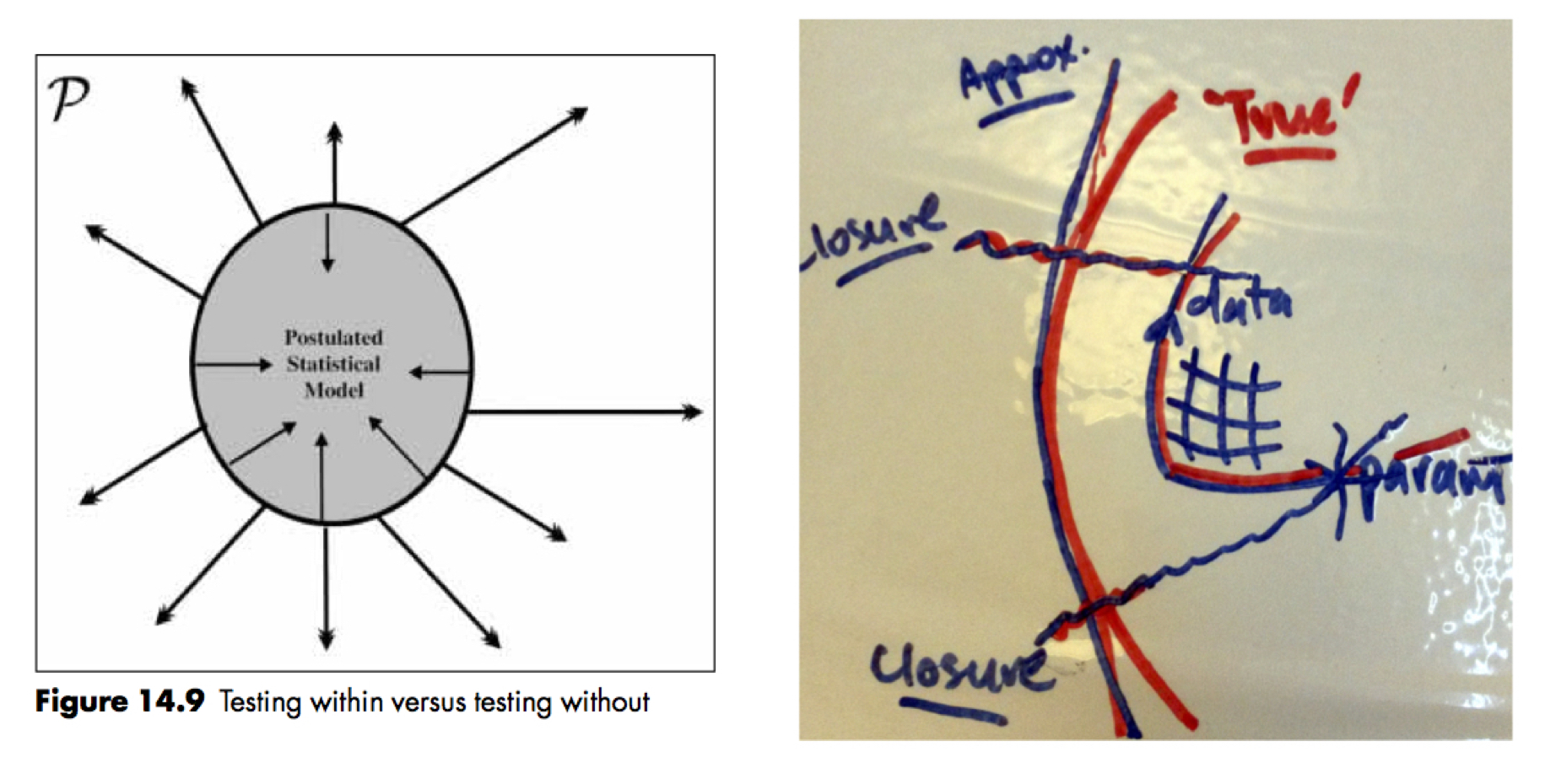
Figure 2: Testing ‘within’ and ‘without’ relative to a model (L; from ‘Probability theory and statistical inference’ by Spanos 1999) and a geometric picture of model closure relative to the ‘truth’ (R; my own drawing).

Each of these figures makes the point that:

even in ‘model world’ (c.f. the ‘real’ world) we need to distinguish between the ‘objective, external’ world and the ‘subjective, internal’ world. In particular, this distinction is drawn relative to the boundary defining the model closure, and applies to both ‘data’ and ‘parameters’.

As I have discussed in other posts, closure is what delinates the boundary between estimating parameters within a model structure and testing the model adequacy with respect to external reality. We have essentially already considered the parameter closure, i.e. discarding ‘irrelevant’ parameters (theoretical constructs). The same idea applies, however, to the data space closure. Some do not distinguish ‘within’ and ‘without’ in the way done here for various reasons – from ‘all models are wrong and therefore subjective’ to leaving ‘lumps of probability‘ to keep the ‘options open’ somewhat. There is some truth in these general ideas; after all, all closures are provisional. I still prefer to explicitly introduce and distinguish ‘inside’ and ‘outside’ a model and ‘objective’ and ‘subjective’ constructs, however – even when both are (and really, can only be) imagined.

‘Intermediate’ structure and multiple scales
On the other hand, a subtle issue emerges in a similar way to in the ‘tacking paradox’ post – the distinction between predictive irrelevance and more ‘complete’ irrelevance, i.e. the presence or absence and nature of further internal degrees of freedom. We need to find a way to follow the advice to

Rule out the accidental features
And you will see: the world is marvellous

– Alexander Block (translated by Sir James Lighthill)

This ‘intermediate’ perspective is described in Barenblatt’s ‘Scaling‘ which quotes the above and also give the following painting as a conceptual example:

Figure 3 “Lincoln in Dalivision, Salvador Dali Lincoln in Dalivision Print, Lincoln in Dalivision”. One (relatively) small scale depicts ‘Gala’ gazing at the sea, which in turn ‘merges into’, at an ‘intermediate’ scale, a portrait of Abraham Lincoln. The ‘frame’ of the full painting ends our ‘boundary of interest’. If we stand much much further back, we no longer recognise any interesting features – our ‘largest’ observation scale determines the largest scale features we wish to perceive.

Related to the (applied mathematics) concepts of intermediate asymptotics and renormalization scaling is another set of concepts that I will (loosely) draw on below – the (thermodynamic) concepts of ‘external variables’, ‘internal variables’ and ‘internal coordinates’. Roughly speaking, the external variables determine the overall ‘shape’ of the closure as determined by ‘background’ conditions and connect our invariant theories (see next) to external measurements, the internal variables are intermediate variables that form (approximately, at least) an invariant and predictively complete set for a (scale-free) phenomenon of interest, while the internal coordinates index a finer set of internal degrees of freedom. In general the internal variables are determined from integrals over internal degrees of freedom/internal coordinates. So we have (at least) three scales – ‘external’, ‘intermediate’ and ‘small’.

This enables us [or will eventually] to compare theories that are a priori distinct, e.g. have different parameter domains and definitions, but seem similar when looked at in the right way. That is, it may be possible to find a common, scale-free predictive theory with a (relatively) invariant set of internal variables that serve as a common target mapping for the variables of distinct theories to enable consistent comparison. To connect back to reality requires ‘boundary closures’ on ‘either side’ of the intermediate, invariant theory – i.e. data space closure via a notion of measurement and parameter space closure via a notion of stability under manipulation/variation in other degrees of freedom (and relates to the formulation of priors).

A basic theme emerges:

‘causality’ and ‘mechanistic’ understanding are about invariant structures under the scales and controls of interest; probability enters into consideration in a somewhat secondary manner: to capture uncertainty within and between structural relationships, and in determining the resolution of control and measurement accuracy.

Additional notes
For now, here are some (very quickly sketched) handwritten notes.

0.0 A first attempt at a ‘closure functor’

0.1 A first/another attempt at relating model closure to ideas of invariance, intermediate asymptotics etc

Further notes
Besides properly tidying these ideas up, I also want to connect them to Laurie Davies’ ‘Approximate models‘ approach.