As mentioned in my previous post I think it makes sense to distinguish parameters from observables (‘data’). What happens if you want to convert between them, however? For example,

what if you want to treat an observable as a fixed or controllable parameter?

The first, intuitive answer is that we should just condition on it using standard probability theory. But we’ve already claimed that observables and parameters should be treated differently – it seems then that there may be a difference between conditioning on an observable, in the sense of probability theory, and treating it as a parameter.

Here then is an unusual, alternative proposal (it is not without precedent, however). As mentioned above, the motivation and distinctions are perhaps subtle – let’s just write some things down instead of worrying too much about these.

Firstly, a non-standard definition to capture what we want to do:

Definition: an ancillary statistic is a statistic (function of the observable data) that is treated as a fixed or controlled parameter.

This is a bit different to the usual definition. No matter.

For one thing

Ancillaries are loved or hated, accepted or rejected, but typically ignored

while (see same link)

Much of the literature is concerned with difficulties that can arise using this third Fisher concept, third after suffciency and likelihood…However, little in the literature seems focused on the continued evolution and development of this Fisher concept, that is, on what modications or evolution can continue the exploration initiated in Fisher’s original papers

So why not mix things up a bit?

Now, given an arbitrary model (family) with parameter ,

we can calculate the distribution of various statistics , and associated joint or conditional distributions in the usual way(s). The conditional distribution of given is defined here as

.

I’ll ignore all measure-theoretic issues.

Now, the above can already be considered a function of and . The question, though, is: is this the right sort of function for treating a statistic as a parameter? Suppose it isn’t. What else can we define? We want to define

as something similar to, but not quite the same as

.

I propose

This ensures that our ancillary statistic is, conceptually at least, actively held fixed for arbitrary , rather than merely coincidentally taking its value. That is, it is an observable treated as a controlled parameter rather than simply a passive, uncontrolled observable.

Addendum
If and are taken to be distinct then what should the latter be called?

Well, I believe this is essentially the same distinction between conditioning and intervening made by Pearl and others. On the other hand, it might be nice to have a term that is a bit more neutral.

Furthermore, this is a distinction that has long been advocated for by a number of likelihood-influenced (if not likelihoodist) and/or frequentist statisticians. It appears Bayesians have been the quickest to blur the distinction – I came across a great example of this recently in an old IJ Good paper. Here is saying he is unable to see the merit in this distinction:

The present post of course claims the distinction is a valuable one.

Now, given the relation to the mathematical notion of a restriction, perhaps this could simply be called t restricted to a, t restricted along a or, to go latin, t restrictus/restrictum/restricta a? 

Rather than conditional inference, should this use of ancillaries instead be called restrictional inference? Or just constrained inference?

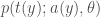
You might also wonder how this connects back to the usual likelihood theory.  For one, as mentioned above, this distinction between types of given has long been made in the likelihood literature. In addition it might be possible to connect the above even more closely to the usual likelihood definitions by considering a generalisation of the above along the lines of (?)

which leads to something like the idea of comparing models along curves of constant ancillary probability. If you are willing to entertain even more structural assumptions, for example a pivotal quantity 

which is a function of both and you can potentially go even further. Such quantities provide an even more explicit bridge between the world of parameters and the world of statistics. Is this further extension, mixing parameters and data even more intimately, necessary or a good idea? I’m not really sure. It seems to me, rather, that ancillaries can get you most of the way without needing to impose or require additional structure on the parameter space.