Version 1.8. (Mostly) written on a phone while Easter shopping.

Likelihood and plausibility 

The usual definition of likelihood takes a probability model family

and defines the likelihood as

For some arbitrary constant C. Note that the data and parameter have switched roles: the likelihood is considered a function of the parameter for fixed data.

A minor modification is to define the ‘unconstrained’ or ‘joint’ likelihood

which is now considered a function of both the parameter and data. Furthermore, a normalisation condition is now a consequence of our definition, rather than somewhat informally added on as in the usual approach. To make this useful, and capable of getting us back to the usual approach as a special case, we define the operation of constraining the likelihood. Importantly, by starting from the joint likelihood, this can be defined in the same manner for both parameter and data.

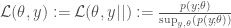
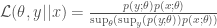
Firstly, constraining on the data gives the usual (normed) likelihood

where we use the notation || to indicate the ‘constraining’ operation. Note also the similarity to the definition of conditional probability (which would require theta to be probabilistic)

The only difference being the use of the ‘sup’ operation vs the integral operation and whether theta is probabilistic or non-probabilistic (in the former case we consider a joint distribution, in the latter a family of distributions).

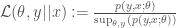
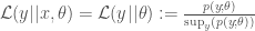
The advantage of this slight generalisation is that we can now we can consider the joint likelihood constrained on the parameter, giving

This is in fact Barndorff-Nielsen’s plausibility function. It can be considered as a measure of self-consistency for a single parameter value (single model instance from the family) and is strongly related to p-value type tests. It does not need alternative parameter values to be considered, rather it needs alternative data to be considered. Clearly it is related in spirit to frequentist concerns of the form ‘what if the data were different?’.

As argued by Barndorff-Nielsen, both aspects give us insight into the problem under consideration – they ask (and hopefully help answer) different questions.

Finally, given the above ‘constraining’ operation, note that our unconstrained likelihood really is just what it says it is – it’s what you get when you ‘constrain on none of the quantities’:

So everything works together as expected.

Extended likelihood and prediction

A related notion, with roots going back quite a few years, clearly explained recently in various places by Pawitan, Lee and Nelder (see e.g. here, here or here as well as references therein for the full history) is extended likelihood. The key twist is allowing random data to be treated as unknown parameters. This helps, for example, for defining a notion of likelihood prediction.

But we already have all the ingredients needed, using the above! Our plausibility function allows the data to be treated as a parameter in a likelihood. It is in essence already a predictive likelihood. 

The above is a slightly different way of looking at these issues than that given by e.g. Pawitan, Lee and Nelder – it is instead based on Barndorff-Nielsen’s ideas mentioned above (which in turn derive from Barnard’s). See also here. On the other hand, the basic idea of extended likelihood is to start from the model family considered as a joint likelihood, so the approach considered here is essentially equivalent (but see future posts on nuisance parameters).

To see how we might incorporate past data, consider a model family

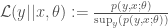
where we suppose x is observed (known) and y is to be predicted (is unknown). So we want to constrain on x and consider y and theta. Consider then

For a fixed choice of theta we would take

Interestingly, in this latter case we learn nothing from past iid samples from the same model instance. That is, for x and y iid from the same fixed model instance (same fixed parameter value) we have

which reduces to (cancelling the x terms)

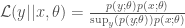
This follows because we are taking theta as fixed and known. We don’t need to use x to estimate theta since we assume it. If instead we use the first expression we get

This allows us to account for our uncertainty in theta and our gain in knowledge about theta from observing x. Now, if the family has constant mode – i.e. if

is the same for all theta, then we have

Note again the similarity to probabilistic updating – the difference is simply that instead of multiplying our model for y by a posterior over theta (based on x) we instead multiply it by a likelihood over theta (based on x). Relatedly, note that our prediction function is the product of two terms. The analogous probabilistic prediction would be based on something like

where instead of the constant mode assumption we need to use something like

i.e. the above is independent of x. Following this aside a bit further, note that if we further marginalised we would get the posterior predictive distribution

but that this is a further reduced form of our (probabilistic) prediction function (Barndorff-Nielsen gives a similar definition for the likelihood prediction function, replacing the integration by maximisation over theta). This indicates to me that there is something to Murray Aitkin’s comments on predictive distributions and his approach summarised here.

Stepping back, note that, in general, all of our main expressions depend on all of the original quantities – no reduction automatically takes place via our constraining operation. We are not removing quantities e.g. via marginalisation or even via maximisation (c.f. the comments on posterior predictive distributions etc). Furthermore no guidance is offered on when or how to choose any particular candidate or set of candidates (like just choosing the max likelihood or set of candidates within some distance from the max likelihood). I’ll look at these issues and some concrete examples next time. These will illustrate the importance of the concepts of independence and orthogonality – whether exact or approximate – for model and/or inferential reduction. I’ll also try to touch on some EDA issues at some point.