Summary
Just a little note on ‘Tropical Bayesian Inference’.

Tropical Bayes and likelihood 
Recently I wrote a short article on the foundations of profile likelihood because I was unsatisfied with the usual descriptions of it as ‘not a real likelihood’. Well, what is it? Why is it so useful (to some)? How should we interpret it? Etc.

It turns out that you can (arguably) think of likelihood in terms of possibility theory, rather than probability theory, and that possibility theory is naturally formulated in terms of the (somewhat obscure) mathematical languages of maxitive measure theory, idempotent probability theory and tropical algebra/tropical geometry.

Once you replace probability by possibility, everything works out basically exactly the same as in standard Bayesian inference. Hence in a recent revision I decided to call it ‘Tropical Bayes’.

You can read the preprint here.

Overview

A short, sketchy and somewhat reluctant note on p-values.

What are p-values for?

One of the key intended uses of p-values is widely acknowledged to be to ‘avoid mistaking noise for signal’. Let’s call this use one.

A related – but distinct – idea is that they are a measure of ‘evidence’. Let’s call this use two.

Evidence?

Richard Royall is among the well-known critics of p-values as evidential measures. On the other hand, he has also written on the concept of ‘misleading evidence’, which appears closely tied to the first use. The short version of his account is that, rather than a p-value, a likelihood ratio should be used as an evidential measure, but that this can also be misleading in individual cases– e.g. it is possible for a particular experiment or study to produce strong but misleading evidence.

In his case this means: a large likelihood ratio arising by chance in a single study. One would not expect this same likelihood ratio to consistently appear in repeated trials.

Apparent signal

More generally, rather than ‘evidence’ let’s call the summary of a particular trial or experiment (or dataset) the ‘apparent signal’. In the terms of my previous post, this is simply the value of an interesting estimator. You have a dataset and notice something interesting; you then summarise this via a ‘statistic’ of some sort.

Importantly, recall that in the previous post we required two things:

• An interesting summary of the given data, and
• An idea of the stability of this summary with respect to ‘similar’ datasets.

Similarly, Royall in fact does make use of what amounts to p-values for characterising this idea of misleading signal. He shows that for two simple hypotheses labelling two probability model instances (with densities) we have

where and are the likelihoods associated with the respective models and indicates that the probability is calculated under the ‘null’ model labelled by 0.

In words: the probability of obtaining an even stronger ‘apparent signal’ (likelihood ratio) under the null model is bounded by the reciprocal of the signal strength (when measuring signal strength in terms of likelihood ratios). This itself is exactly what a p-value is intended to do.

Signal stability vs strength

It appears then that the role of the p-value is best thought of as characterising the stability of the apparent signal rather than the apparent signal itself.

For example, it is perfectly possible to have a strong but unstable apparent signal. This is also known as ‘overfitting’. Or, a weak but stable signal: a small but consistent ‘effect’.

I would argue that the ‘effect estimate’ itself should be used as the ‘evidential’ measure (if such a measure is desired – I have generally come to prefer to think in different terms, but this is the nearest translation I can offer). This is also a natural consequence of Royall’s argument, but separated from dependence on the likelihood ratio.

So, a larger ‘effect estimate’ is itself greater ‘evidence’ against the null. This is also more naturally compatible with ‘approximation’-based thinking (I think!): a larger effect estimate is a greater indication of the inadequacy of the null as a good approximate model.

A key here is the tension between the ‘signal’ component, e.g. the estimated mean value say, and the ‘noise’ component e.g. the variability of this. It is the signal that measures ‘evidence’ (or whatever you want to call it); the variability measures the stability of this.

Measuring apparent signal

If the p-value measures the stability of an apparent signal but not the strength as such, how exactly should we measure strength? As mentioned I think we need to use the ‘effect estimate’ itself (and more generally direct ‘statistics of interest’ calculated from the data) as the natural measures of ‘interestingness’ or ‘signal’. Note though that this requires an idea of ‘how large of an effect is interesting’ independently of its probability under the null.

Royall’s proposal is to report the likelihood ratio between the null and an interesting comparison hypothesis. While I now doubt the generality of the likelihood ratio approach (and likelihood-based approaches in general) this again illustrates the important point: your statistic/estimator/apparent signal measure should reflect what is of interest to the analyst and usually requires more than just a null. In essence this is because a ‘null’ consists of ‘zero signal’ and an assumed ‘noise’ model. We want to know what ‘non-zero signal’ should look like.

Comparative choice dilemma

A big issue is when the problem is framed as having to choose between only two discrete models (i.e. between two simple hypotheses). This raises an issue because it could be the case that neither model is a good fit but one is still a much ‘better’ fit than the other. This is a potential problem for the idea of ‘comparative’ testing/evidence.

In this case one faces a tension: if you use a test statistic or ‘apparent signal’ measure that only compares the null to the data then you may reject it. If you then implicitly embed this into a comparative/two model choice problem then you are automatically ‘accepting the alternative’. But this may itself be a bad model. It could even be a worse model.

One ‘solution’, if you must phrase it as a comparative choice problem, is to include both models in the test statistic itself. This is what is done when the likelihood ratio is used as the test statistic. Thus the likelihood ratio measures the ‘comparative evidence’ or ‘comparative apparent signal’ while the p-value for this likelihood ratio measures the probability of this being a misleading signal.

In short:

• Your statistic captures what you mean by interesting, so anything you are interested in (e.g. alternative hypotheses, effect sizes of interest etc) should be included here. It should be expressed in units of relevance to the problem and this is not generally ‘probability’.

• A p-value is one way of summarising the stability of your statistic of interest, under ‘null variations’. It does not itself measure interestingness.

Overview/disclaimer: Can you do (semi-formal) statistics without assuming, even ‘temporarily’ that a model is ‘true’? Can estimation be done without implying an equivalent hypothesis testing formulation? Here’s a very rough sketch of one attempt. The account is, I hope, mostly a ‘positive’ proposal rather than a critique of existing practice. You have to look for the notes that aren’t played to see the ‘negative’ side/critique…

What is (formal/semi-formal) statistics? A modification of Fisher: Statistics is the study of data, measurements and/or individuals in aggregation.

We call these things that statistics studies ‘aggregates’, ‘datasets’ or ‘populations’ for short. Data in aggregation, i.e. populations, can possess properties distinct from unaggregated data, i.e. individuals. This is an important, if often neglected, feature of statistics: see e.g. Simpson’s paradox, ecological fallacies etc. Also note that in our case a finite sample is a valid aggregate or population in and of itself (but adding more data of course produces a new aggregate distinct from the original).

Statistics aims to both summarise and quantify aggregates and to account for the variation in these summaries across different aggregates. In particular, a statistic, estimator or learning map (we consider these to be different names for the same thing) is a function designed with the purpose of reducing aggregates (lying in the function’s domain) to a summary (lying in the function’s range).

Here we call the space within which these functions take values parameter space, and the domain containing populations/aggregates the data space.

We use the term ‘parameter space’ regardless of whether the output values of the estimator map are ‘model labels’/parameters of models, whether they represent values of an estimator evaluated at a ‘true population’ (which we don’t assume exists) or neither of these. They do not need to be real-valued either – they can be e.g. function-valued, density-valued, image-valued etc.

A common example of an estimator is mapping a set of non-co-linear (x,y) pairs to a straight line summary. This can be obtained by a formal process such as minimising a least-squares criterion or more informally such as drawing a line by hand but should, I would argue, give the same output given the same input (i.e. be deterministic; stochastic estimators can be represented by deterministic but measure-valued functions). A less typical example would be to map a picture of a human face to an emoji, in which case the estimator is emoji-valued.

The important thing in practice is that the resulting ‘parameter’ should represent a reduction of the data population and be an informative or interesting summary of the data. What is ‘interesting’ is judged by the scientists studying the subject but, because of the nature of the aggregation process, this often takes a common form across particular discipline boundaries – e.g. a mean or mode (of a population of numerical measurements) can be interesting in a variety of situations. A related phenomonen is what physicsts call ‘universality’.

Again, the domains of these functions are populations (aggregations) and the ranges are interesting summaries (often, but not always, real-valued).

The purpose of an estimator, considered as a function of datasets, is to

a) provide a useful/informative/interesting (to the analyst) reduction of a given dataset/aggregation (e.g. (x,y) pairs to a straight line) and to

b) be a stable reduction in the sense that when evaluated on ‘similar’ datasets (input) it gives a ‘similar’ output (estimate value).

‘Similar’ is a semi-formal concept typically defined by examples and procedures. A common way to illustrate the meaning of a ‘similar dataset’ is via resampling and related procedures such as bootstrapping, jackknifing, data splitting, data perturbation etc. in which an analyst gives a constructive procedure, illustrating what they mean by ‘similar dataset’, which produces new example datasets given a starting example dataset. One could potentially define this slightly more formally as a (often stochastic/probabilistic) mapping from example datasets to new example datasets, but the mapping must be provided by the analyst. A dataset may also include ‘regime indicators’ representing partially recorded information, and similarity measures can include differences in these.

The notion of similar is also made more concrete by introducing an explicit metric, distance and/or topology on examples: examples are more similar the closer they are in distance and more dissimilar the further they are away in distance. The notion of distance should be chosen to accurately reflect the analyst judgements of ‘similar’ as above; however, as before, some distances have wide applicability due to the nature of aggregations: e.g. certain statistical distances like the Kolmogorov metric capture useful notions of probabilistic convergence.

A stable estimator is one which produces estimates (summaries) of ‘similar’ datasets that are also ‘similar’ in a quantitative (or qualitative) sense. This requires another notion of ‘similar’ for parameter space (the output/range space of estimators). This is perhaps most usefully carried out by defining two metrics and/or topologies – one for data space and one for parameter space. In this way, stable means, in essence, that the estimator is a continuous function between these two spaces.

Directly plotting the estimator values (when possible to plot) obtained from a variety of ‘similar’ datasets is a useful way to visualise its stability/instability. This is similar to a ‘sampling distribution’ in frequentist statististics but need not have this interpretation. Instead I suggest the term distribution of variation.

Stability has the ‘predictive’ consequence that, if future datasets are ‘similar’ to the current dataset in the sense defined above, then the estimator evaluated on the present dataset is, by definition, similar to the estimate that would be found by evaluating the estimator on future datasets.

If, however, future datasets are not similar in the sense considered by the analyst then there is no guarantee of stability and/or prediction. Stability/continuity wrt a chosen notion of similarity is the feature that dictates predictive guarantees.

‘Overfitting’ is a form of instability that results from inadequate attention to defining stability wrt ‘similar’ datasets and focusing too much on one particular dataset. Instability implies overfitting and overfitting implies instability. Prediction can only be reliably guaranteed when the future is ‘similar’ to the past in a specified sense and estimators are designed with this similarity in mind.

Overfitting is prevented, to the extent that it is possible, by ensuring the estimator is stable with respect to similar datasets. Of course, it must also provide an ‘interesting’ summary of the present dataset – e.g. mapping everything to zero is stable but uninteresting.

This leads to a trade-off which here is just another form of what is called the bias-variance trade-off in statistical machine learning. The particular trade-off between ‘bias’ and ‘variance’ in SML theory is just one example of what is a somewhat more general and ‘universal’ phenomenon, however.

In short: in general the amount of information retained by an estimator when evaluated on a given dataset ‘conflicts with’ or ‘trades-off against’ the stability of this estimator when evaluated on other ‘similar’ but distinct datasets. Statistics is about determining data reductions (estimators) that balance retaining interesting information and stability.

A grab bag of somewhat related reading

Tukey, J.W. (1997). More honest foundations for data analysis. Journal of Statistical Planning and Inference, 57(1), 21-28. (h/t C. Hennig).

Tukey, J.W. (1993). Issues relevant to an honest account of data-based inference, partially in the light of Laurie Davies’ paper. Princeton University, Princeton. (link)

Davies, P.L., (2014). Data analysis and approximate models: Model choice, Location-Scale, analysis of variance, nonparametric regression and image analysis. CRC Press.

Poggio, T., Rifkin, R., Kukherjee, S., & Niyogi, P. (2004). General conditions for predictivity in learning theory. Nature, 428(6981), 419.

Liu, K., & Meng, X. L. (2016). There Is Individualized Treatment. Why Not Individualized Inference?. Annual Review of Statistics and Its Application 3:1, 79-111.

Version 1.8. (Mostly) written on a phone while Easter shopping.

Likelihood and plausibility 

The usual definition of likelihood takes a probability model family

and defines the likelihood as

For some arbitrary constant C. Note that the data and parameter have switched roles: the likelihood is considered a function of the parameter for fixed data.

A minor modification is to define the ‘unconstrained’ or ‘joint’ likelihood

which is now considered a function of both the parameter and data. Furthermore, a normalisation condition is now a consequence of our definition, rather than somewhat informally added on as in the usual approach. To make this useful, and capable of getting us back to the usual approach as a special case, we define the operation of constraining the likelihood. Importantly, by starting from the joint likelihood, this can be defined in the same manner for both parameter and data.

Firstly, constraining on the data gives the usual (normed) likelihood

where we use the notation || to indicate the ‘constraining’ operation. Note also the similarity to the definition of conditional probability (which would require theta to be probabilistic)

The only difference being the use of the ‘sup’ operation vs the integral operation and whether theta is probabilistic or non-probabilistic (in the former case we consider a joint distribution, in the latter a family of distributions).

The advantage of this slight generalisation is that we can now we can consider the joint likelihood constrained on the parameter, giving

This is in fact Barndorff-Nielsen’s plausibility function. It can be considered as a measure of self-consistency for a single parameter value (single model instance from the family) and is strongly related to p-value type tests. It does not need alternative parameter values to be considered, rather it needs alternative data to be considered. Clearly it is related in spirit to frequentist concerns of the form ‘what if the data were different?’.

As argued by Barndorff-Nielsen, both aspects give us insight into the problem under consideration – they ask (and hopefully help answer) different questions.

Finally, given the above ‘constraining’ operation, note that our unconstrained likelihood really is just what it says it is – it’s what you get when you ‘constrain on none of the quantities’:

So everything works together as expected.

Extended likelihood and prediction

A related notion, with roots going back quite a few years, clearly explained recently in various places by Pawitan, Lee and Nelder (see e.g. here, here or here as well as references therein for the full history) is extended likelihood. The key twist is allowing random data to be treated as unknown parameters. This helps, for example, for defining a notion of likelihood prediction.

But we already have all the ingredients needed, using the above! Our plausibility function allows the data to be treated as a parameter in a likelihood. It is in essence already a predictive likelihood. 

The above is a slightly different way of looking at these issues than that given by e.g. Pawitan, Lee and Nelder – it is instead based on Barndorff-Nielsen’s ideas mentioned above (which in turn derive from Barnard’s). See also here. On the other hand, the basic idea of extended likelihood is to start from the model family considered as a joint likelihood, so the approach considered here is essentially equivalent (but see future posts on nuisance parameters).

To see how we might incorporate past data, consider a model family

where we suppose x is observed (known) and y is to be predicted (is unknown). So we want to constrain on x and consider y and theta. Consider then

For a fixed choice of theta we would take

Interestingly, in this latter case we learn nothing from past iid samples from the same model instance. That is, for x and y iid from the same fixed model instance (same fixed parameter value) we have

which reduces to (cancelling the x terms)

This follows because we are taking theta as fixed and known. We don’t need to use x to estimate theta since we assume it. If instead we use the first expression we get

This allows us to account for our uncertainty in theta and our gain in knowledge about theta from observing x. Now, if the family has constant mode – i.e. if

is the same for all theta, then we have

Note again the similarity to probabilistic updating – the difference is simply that instead of multiplying our model for y by a posterior over theta (based on x) we instead multiply it by a likelihood over theta (based on x). Relatedly, note that our prediction function is the product of two terms. The analogous probabilistic prediction would be based on something like

where instead of the constant mode assumption we need to use something like

i.e. the above is independent of x. Following this aside a bit further, note that if we further marginalised we would get the posterior predictive distribution

but that this is a further reduced form of our (probabilistic) prediction function (Barndorff-Nielsen gives a similar definition for the likelihood prediction function, replacing the integration by maximisation over theta). This indicates to me that there is something to Murray Aitkin’s comments on predictive distributions and his approach summarised here.

Stepping back, note that, in general, all of our main expressions depend on all of the original quantities – no reduction automatically takes place via our constraining operation. We are not removing quantities e.g. via marginalisation or even via maximisation (c.f. the comments on posterior predictive distributions etc). Furthermore no guidance is offered on when or how to choose any particular candidate or set of candidates (like just choosing the max likelihood or set of candidates within some distance from the max likelihood). I’ll look at these issues and some concrete examples next time. These will illustrate the importance of the concepts of independence and orthogonality – whether exact or approximate – for model and/or inferential reduction. I’ll also try to touch on some EDA issues at some point.

…can be found here: https://github.com/omaclaren/open-learning-material

As mentioned there

Like all such material much of it is either shamelessly (or shamefully!) plagiarised, borrowed, edited etc from other sources, especially courses I’ve taken before or notes I’ve inherited from past lecturers. I will try to add some credits as I go. This is essentially impossible for some material, however, as it was effectively picked up from the aether.

If you have any objections to me making this material (or some parts of it) available then let me know. My intention is simply to make it available for anyone who wants to learn about these topics.

Also, this material should be assumed to contain at least some gross errors or major misconceptions!

At the moment it includes material on partial differential equations, probability, Markov processes and qualitative analysis of differential equations.

I’m working on improving the material (and adding more) so expect it to change. In particular I’m currently updating the material on qualitative analysis of differential equations. I’m hoping to better balance the (interesting!) underlying theory with more emphasis on, and examples of, simple and direct applications of the theory.

As mentioned in my previous post I think it makes sense to distinguish parameters from observables (‘data’). What happens if you want to convert between them, however? For example,

what if you want to treat an observable as a fixed or controllable parameter?

The first, intuitive answer is that we should just condition on it using standard probability theory. But we’ve already claimed that observables and parameters should be treated differently – it seems then that there may be a difference between conditioning on an observable, in the sense of probability theory, and treating it as a parameter.

Here then is an unusual, alternative proposal (it is not without precedent, however). As mentioned above, the motivation and distinctions are perhaps subtle – let’s just write some things down instead of worrying too much about these.

Firstly, a non-standard definition to capture what we want to do:

Definition: an ancillary statistic is a statistic (function of the observable data) that is treated as a fixed or controlled parameter.

This is a bit different to the usual definition. No matter.

For one thing

Ancillaries are loved or hated, accepted or rejected, but typically ignored

while (see same link)

Much of the literature is concerned with difficulties that can arise using this third Fisher concept, third after suffciency and likelihood…However, little in the literature seems focused on the continued evolution and development of this Fisher concept, that is, on what modications or evolution can continue the exploration initiated in Fisher’s original papers

So why not mix things up a bit?

Now, given an arbitrary model (family) with parameter ,

we can calculate the distribution of various statistics , and associated joint or conditional distributions in the usual way(s). The conditional distribution of given is defined here as

.

I’ll ignore all measure-theoretic issues.

Now, the above can already be considered a function of and . The question, though, is: is this the right sort of function for treating a statistic as a parameter? Suppose it isn’t. What else can we define? We want to define

as something similar to, but not quite the same as

.

I propose

This ensures that our ancillary statistic is, conceptually at least, actively held fixed for arbitrary , rather than merely coincidentally taking its value. That is, it is an observable treated as a controlled parameter rather than simply a passive, uncontrolled observable.

Addendum
If and are taken to be distinct then what should the latter be called?

Well, I believe this is essentially the same distinction between conditioning and intervening made by Pearl and others. On the other hand, it might be nice to have a term that is a bit more neutral.

Furthermore, this is a distinction that has long been advocated for by a number of likelihood-influenced (if not likelihoodist) and/or frequentist statisticians. It appears Bayesians have been the quickest to blur the distinction – I came across a great example of this recently in an old IJ Good paper. Here is saying he is unable to see the merit in this distinction:

The present post of course claims the distinction is a valuable one.

Now, given the relation to the mathematical notion of a restriction, perhaps this could simply be called t restricted to a, t restricted along a or, to go latin, t restrictus/restrictum/restricta a? 

Rather than conditional inference, should this use of ancillaries instead be called restrictional inference? Or just constrained inference?

You might also wonder how this connects back to the usual likelihood theory.  For one, as mentioned above, this distinction between types of given has long been made in the likelihood literature. In addition it might be possible to connect the above even more closely to the usual likelihood definitions by considering a generalisation of the above along the lines of (?)

which leads to something like the idea of comparing models along curves of constant ancillary probability. If you are willing to entertain even more structural assumptions, for example a pivotal quantity 

which is a function of both and you can potentially go even further. Such quantities provide an even more explicit bridge between the world of parameters and the world of statistics. Is this further extension, mixing parameters and data even more intimately, necessary or a good idea? I’m not really sure. It seems to me, rather, that ancillaries can get you most of the way without needing to impose or require additional structure on the parameter space.

Bayesian inference is useful. It also provides a ‘quick and dirty‘ route to thinking about statistical inference since it just uses basic probability theory. This is to me its biggest strength and weakness – the ‘everything is probability theory’ view.
Why isn’t everything probability theory? In short

• Not everything is a ‘sum to one’ game
• Both uncertainty (‘randomness’) and structure are important

Regarding the first point, I think it makes sense to have a notion of ‘observable’ for which mutually exclusive possibilities must ‘sum to one’ – you either observe a head or observe a tail, for example.

One the other hand, I think it makes sense to include a notion of quantity for which the mutually exclusive possibilities do not need to sum to one. Two distinct models can be equally consistent with given observations. Introducing a third distinct model, also equally consistent with observations, shouldn’t change the ‘possibility’ value of the first two. It does change the probability of the first two, however.

These ‘purely possibilistic’ quantities are what I would call parameters. Probabilistic quantities are observables or ‘data’.

Interestingly, the key difference between likelihood and probability is that the former need not sum to one. Probability applies to data, likelihood to parameters. In certain special cases we can strengthen from likelihood to probability and regain Bayes (or perhaps confidence/fiducial) – identifiable models being one requirement. In less well-constrained problems I prefer likelihood.

The second issue is how to represent structure in addition to uncertainty. For example, a probability distribution is assigned in a given context. How does that probability distribution change when we change context? This is in a sense ‘external’ or ‘structural’ information. You can kludge it within Bayes using ‘conditioning on background information’ but this background information typically does not require a probability distribution. It is instead usually more akin to a ‘possibilistic’ quantity under analyst control or subject to assumptions external to the probability distribution. That is, it is ‘prior information’ but it does not take the form of a probability distribution. This is more common than you would think from the usual Bayesian story.

For example, Pearl – a self-described ‘half-Bayesian’ (perhaps even less these days) –  uses ‘do’ notation to distinguish some types of structural assumption from the merely ‘seen’ observables described by probability. Likelihood can also incorporate these assumptions somewhat more naturally than Bayes as it allows for non-probabilistic ‘possibilistic’ quantities.

Compare Pearl’s

p(y|x,do(z))

to the likelihood (and frequentist) notation

p(y|x;z)

In this case z, and the dependence of each p(y|x) on z, lies outside the probability model. That is, the above represents an indexed family of probability distributions

z->p(y|x),

no prior over z required.

An even more subtle ‘structural’ issue is the question of how ‘raw’ data obtains semantics or meaning. This to me is a point where both likelihood and probability/Bayes are open to criticism. Luckily, some of Fisher’s original ideas on, and motivations for, sufficiency and ancillarity can be used to improve the likelihood approach. I think. But that’s a topic for another day!

Postscript
These might seem like purely philosophical concerns but to me they are quite practical. In short – and contra Lindley – I don’t think Bayesian inference works very well in the presence of non-identifiability. I’ll try to illustrate with some examples at some point.

It’s also worth noting that one of Neyman’s goals (see the discussions at the end of this) was “to construct a theory of mathematical statistics independent of the conception of likelihood…entirely based on the classical theory of probability.” Albeit in a different manner to Bayesian inference. This led him to “the basic conception…of frequency of errors in judgment”. I think such ‘error statistical’ frequentist inference also suffers some similar issues in dealing with non-identifiable problems.

Overview/motivation
The interpretation of logical quantifiers such as ‘there exists‘ and ‘for all‘ and the associated ontological implications of these interpretations is (apparently – or at least it was) an important topic in philosophy. I encountered these interpretations a few years ago when reading Haack’s ‘Philosophy of Logics’, but didn’t pay much attention. Quine is a central figure here – e.g. his famous (within philosophy, anyway) saying ‘to be is to be the value of a variable‘ concerns this issue.

I realised recently that I’ve been thinking about somewhat similar issues, albeit in a more ‘applied’ context, e.g. when talking about the interpretation of ‘for all’ in formulating ‘schematic’ model closure assumptions (see here). So, here a few notes on the topic. The obvious disclaimer applies – I am not a philosopher. I’m just hoping to get a few basic conceptual ideas straightened out in my head, so that I may better formalise some arguments useful in science and statistics. I am not aiming to ‘solve’ the general philosophical problems! Corrections or comments welcome.

The problem
Here is a brief sketch of the issue as it arises for the existential quantifier. The question is: how should we interpret statements of quantified logic of the form

We have (or there exists??), in fact, two options.

Objectual: There exists an object x such that it has property P.

Substitutional: There exists an instance of a statement having the general form P(x), obtained by substituting some name, term or expression etc for x, that is true.

In the former, the emphasis is placed on objects and their possession of properties, in the latter, the emphasis is placed on statement forms and the truth of particular statement instances.

In particular, in the latter, substitutional, case truth is a property of statements ‘as a whole’ and need not relate to ‘actual objects’ occurring in the sentence.

The classic example is that, on the objectual reading,

(S): Pegasus is a flying horse

can be taken to mean

(S via Obj.): “There exists an object (e.g. Pegasus) which is both a horse and can fly”

We would normally take this as false, since no such object ‘really exists’. On the other hand, on the substitutional reading we may take this to mean

(S via Subs.): There is a true statement of the form ‘x is a flying horse’ (e.g. Pegasus is a flying horse)

The justification for taking this as true is that, given our knowledge of mythology (certainly a real subject itself), we may take this to express a true statement without further commitment to (or even ‘attention to’) the existence of the ‘objects’ or ‘properties’ involved.

Thus the substitutional interpretation refers to the truth or falsity of resultant sentences/statements ‘as a whole’ (and the forms of such sentences/statements), while the objectual intepretation refers to the existence of objects with properties, and hence in a sense gives a more ‘granular’ interpretation.

Both seem to me to involve subtle issues of context, however – e.g. we can presumably only interpret the above statement instance as ‘true’ in the substitutional interpretation given the context of mythology.

Marcus and Kripke offered defenses of the substitutional interpretation while Quine advocated the objectual interpretation (hence ‘to be is to be the value of a variable’).

There is obviously much more to this topic – see e.g. Haack’s book, the SEP. For now, I note that I find myself reasonably sympathetic to the substitutional interpretation (or perhaps both interpretations, depending on the circumstances). This appears to be roughly consistent with what I was attempting to express here.

There also seems to be something here that depends on whether, given the ‘function’ P(x), we focus on the ‘domain of naming’ or on the ‘codomain of statements’. These issues hence also seem to connect with the issue of how to interpret (proper) names e.g. as ‘mere tags’ (Marcus), ‘rigid designators’ (Kripke), ‘definite descriptions’ (Russell) or as ‘predicates’ (Quine). The substitutional interpretation is generally allied with the view of proper names as ‘mere tags’ or as ‘rigid designators’, and I have become quite fond of (what I understand by) this idea. It would be too much to go into this in any detail at the moment, however.

Another short (and simple) note on the so-called tacking paradox from the philosophy of science literature. Continuing on from here and related to a recent blog comments exchange here. See those links for the proper background.

[Disclaimer: written quickly and using wordpress latex haphazardly with little regard for aesthetics…]

Consider a scientific theory with two ‘free’ or ‘unknown’ parameters, a and b say. This theory is a function which outputs predictions . I will assume this is a deterministic function for simplicity.

Suppose further that each of the parameters is discrete-valued and can take values in . Assuming that there is no other known constraint (i.e. they are ‘variation independent’ parameters) then the set of possible values is the set of all pairs of the form

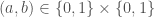
That is, . Just to be simple-minded let’s arrange these possibilities in a matrix giving

This leads to a set of predictions for each possibility, again arranged in a matrix

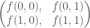
Now our goal is to determine which of these cases are consistent with, supported by and/or confirmed by some given data (measured output) .

Suppose we define another function of these two parameters to represent this and call it for ‘consistency of’ or, if you are more ambitious, ‘confirmation of’ any particular pair of values with respect to the observed data .

For simplicity we will suppose that outputs a definite value which can be definitively compared to the given . We will then require iff , and otherwise. That is, it outputs 1 if the predictions given and values match, 0 if the predictions do not. Since will be fixed here I will drop , i.e. I will use without reference to .

Now suppose that we find the following results for our particular case

How could we interpret this? We could say e.g. and are ‘confirmed/consistent’ (i.e. ), or we could shorten this to say is confirmed for any replacement of the second argument. Clearly this corresponds to a case where the first argument is ‘doing all the work’ in determining whether or not the theory matches observations.

Now the ‘tacking paradox’ argument is essentially:

so

is confirmed, i.e. ‘a=0 & b=0’ is confirmed. But ‘a=0 & b=0’ logically implies ‘b=0’ so we should want to say ‘b=0’ is confirmed. But we saw

and so

is also confirmed, which under the same reasoning gives that ‘b=1’ is confirmed!

Contradiction!

There are a number of problems with this argument, that I would argue are particularly obscured by the slip into simplistic propositional logic reasoning.

In particular, we started with a clearly defined function of two variables . Now, we found that in our particular case we could reduce some statements involving to an ‘essentially’ one argument expression of the form ‘‘ or ‘ is confirmed’, i.e. we have confirmation for a=0 and b ‘arbitrary’. This is of course just ‘quantifying’ over the second argument – we of course can’t leave any free (c.f. bound) variables. But then we are led to ask

What does it mean to say ‘b is confirmed’ in terms of our original givens?

Is this supposed to refer to ? But this is undefined – is of course a function of two variables. Also, b is a free (unbound) variable in this expression. Our previous expression had one fixed and one quantified variable, which is different to having a function of one variable.

OK – what about trying something similar to the previous case then? That is, what about saying ? But this is a short for a claim that both and hold (or that their conjunction is confirmed, if you must). This is clearly not true. Similarly for .

So we can clearly see that when our theory and hence our ‘confirmation’ function is a function of two variables we can only ‘localise’ when we spot a pattern in the overall configuration, such as our observation that holds.

So, while the values of the C function (i.e. the outputs of 0 and 1) are ordered (or can be assumed to be), this does not guarantee a total order when it is ‘pulled back’ to the parameter space. That is, does not guarantee an ordering on the parameter space that doesn’t already admit an ordering! It also doesn’t allow us to magically reduce a function of two variables to a function of one without explicit further assumptions. Without these we are left with ‘free’ (unbound) variables.

This is essentially a type error – I take a scientific theory (here) to be a function of the form

,

i.e a function from a two-dimensional ‘parameter’ (or ‘proposition’) space to a (here) one dimensional ‘data’ (or ‘prediction’, ‘output’ etc) space. The error (or ‘paradox’) occurs when taking a scientific theory to be simply a pair

,

rather than a function defined on this pair.

That is, the paradox arises from a failure to explicitly specify how the parameters of the theory are to be evaluated against data, i.e. a failure to give a ‘measurement model’.

(Note: Bayesian statistics does of course allow us to reduce a function of two variables to one via marginalisation, and given assumptions on correlations, but this process again illustrates that there is no paradox; see previous posts).

One objection is to say – “well this clearly shows a ‘logic’ of confirmation is impossible”. Staying agnostic with respect to this response, I would instead argue that what it shows is that:

The ‘logic’ of scientific theories cannot be a logic only of ‘one-dimensional’ simple propositions. A scientific theory is described at the very, very minimum by a ‘vector’ of such propositions (i.e. by a vector of parameters), which in turn lead to ‘testable’ predictions (outputs from the theory). That is, scientific theories are specified by multivariable functions. To reduce such functions of collections of propositions, e.g. a function f(a,b) of a pair (a,b) of propositions, to functions of less propositions, e.g. ‘f(a)’, requires the use – again at very, very minimum, of quantifiers over the ‘removed’ variables, e.g. ‘f(a,b) = f(a,-) for all choices of b’.

Normal probability theory (e.g the use of Bayesian statistics) is still a potential candidate in the sense that it extends to the multivariable case and allows function reduction via marginalisation. Similarly, pure likelihood theory involves concepts like profile likelihood to reduce dimension (localise inferences). While standard topics of discussion in the statistical literature (e.g. ‘nuisance parameter elimination’), this all appears to be somewhat overlooked in the philosophical discussions I’ve seen.

So this particular argument is not, to me, a good one against Bayes/Likelihood approaches.

(I am, however, generally sympathetic to the idea that functions like that above are better considered as consistency functions rather than as confirmation functions – in this case the, still fundamentally ill-posed, paradox ‘argument’ is blocked right from the start since it is ‘reasonable’ for both ‘b=0’ and ‘b=1‘ to be consistent with observations. On the other hand it is still not clear how you are supposed to get from a function of two variables to a function of one. Logicians may notice that there are also interesting similarities with intuitionistic/constructive logic see here or here and/or modal logics, see here – I might get around to discussing this in more detail someday…)

To conclude: the slip into the language of simple propositional logic, after starting from a mathematically well-posed problem, allows one to ‘sneak in’ a ‘reduction’ of the parameter space, but leaves us trying to evaluate a mathematically undefined function like .

The tacking ‘paradox’ is thus a ‘non-problem’ caused by unclear language/notation.

Addendum – recently, while searching to see if people have made similar points before, I came across this nice post ‘Probability theory does not extend logic‘. 

The basic point is that while probability theory uncontroversially ‘extends’ what I have called simple ‘one-dimensional’ propositional logic here, it does not uncontroversially extend predicate logic (i.e. the basic logical language required for mathematics, which uses quantifiers) nor logic involving relationships between quantities requiring considerations ‘along different dimensions’. 

While probability theory can typically be made to ‘play nice’ with predicate logic and other systems of interest it is important to note that it is usually the e.g. predicate logic or functional relationships – basically, the rest of mathematical language – doing the work, not the fact that we replace atomic T/F with real number judgements. Furthermore the formal justifications of probability theory as an extension of logic used in the propositional case do not translate in any straightforward way to these more complicated logical or mathematical systems.

Interestingly for the Cox-Jaynesians, while (R.T.) Cox appears to have been aware of this, and he even considered extensions involving ‘vectors of propositions’ – leading to systems which no longer satisfy all the Boolean logic rules (see e.g. the second chapter of his book) – Jaynes appears to have missed the point (see e.g. Section 1.8.2 of his book). As hinted at above, some of the ambiguities encountered are potentially traceable – or at least translatable – into differences between classical and constructive logic. Jaynes also appears to have misunderstood the key issues here, but again that’s a topic for another day.

Now all of this is not to say that Bayesian statistics as practiced is either right or wrong but that the focus on simple propositional logic is the source of numerous confusions on both sides. 

Real science and real applications of probability theory involve much more than ‘one-dimensional’ propositional logic. Addressing these more complex cases involves numerous unsolved problems.

This is ‘Not a Research Blog’, but nevertheless some thoughts on, and application of, hierarchical Bayes that are related to what I’ve been posting about here can be found in my recent preprint:

A hierarchical Bayesian framework for understanding the spatiotemporal dynamics of the intestinal epithelium

A few comments. I actually wrote essentially all of this about a year ago. The quirks of interdisciplinary research mean, however, that I have only just recently been able to post even a preprint of this work online (data/other manuscript availability issues etc). Some of my views may have changed slightly since then – but probably not overly much (and most of the more different ideas would relate to alternative frameworks rather than modifications of the present approach). Of course the usual delays of publication mean this happens fairly often – yet another reason for using preprints. This was also my first bioRxiv submission (bioRvix is essentially arXiv targeted specifically at biology and biological applications) – it was extremely easy to use and went through screening in less than a day.

This manuscript was also a first attempt to pull together a lot of ideas I’d been playing around with relating to hierarchical models, statistical inference, prediction, evidence, causality, discrete vs continuum mechanistic models, model checking etc, and apply them to a real problem with real data. As such it’s reasonably long, but I think readable enough. In some ways it probably reads more like a textbook, but some might find that useful so I’ve tried to frame that as a positive.